Understand continuous aggregates

Continuous aggregates automatically precompute and store aggregate data for lightning-fast queries on time-series data in TimescaleDB

In modern applications, data usually grows very quickly. This means that aggregating it into useful summaries can become very slow. If you are collecting data very frequently, you might want to aggregate your data into minutes or hours instead. For example, if an IoT device takes temperature readings every second, you might want to find the average temperature for each hour. Every time you run this query, the database needs to scan the entire table and recalculate the average. makes aggregating data lightning fast, accurate, and easy with continuous aggregates.

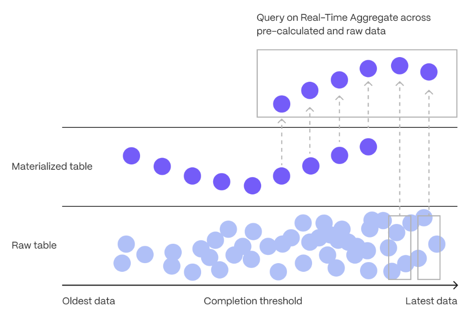
Continuous aggregates in are a kind of hypertable that is refreshed automatically in the background as new data is added, or old data is modified. Changes to your dataset are tracked, and the hypertable behind the continuous aggregate is automatically updated in the background.

Continuous aggregates have a much lower maintenance burden than regular materialized views, because the whole view is not created from scratch on each refresh. This means that you can get on with working your data instead of maintaining your database.

Because continuous aggregates are based on hypertables, you can query them in exactly the same way as your other tables. This includes continuous aggregates in the rowstore, compressed into the columnstore, or tiered to object storage. You can even create continuous aggregates on top of your continuous aggregates, for an even more fine-tuned aggregation.

Real-time aggregation enables you to combine pre-aggregated data from the materialized view with the most recent raw data. This gives you up-to-date results on every query.

Types of aggregation

There are three main ways to make aggregation easier: materialized views, continuous aggregates, and real-time aggregates.

• Materialized views are a standard function. They are used to cache the result of a complex query so that you can reuse it later on. Materialized views do not update regularly, although you can manually refresh them as required.

• Continuous aggregates are a -only feature. They work in a similar way to a materialized view, but they are updated automatically in the background, as new data is added to your database. Continuous aggregates are updated continuously and incrementally, which means they are less resource intensive to maintain than materialized views. Continuous aggregates are based on hypertables, and you can query them in the same way as you do your other tables.

• Real-time aggregates are a -only feature. They are the same as continuous aggregates, but they add the most recent raw data to the previously aggregated data to provide accurate and up-to-date results, without needing to aggregate data as it is being written.

In v2.13 and later, real-time aggregates are DISABLED by default. In earlier versions, real-time aggregates are ENABLED by default; when you create a , queries to that view include the results from the most recent raw data.

Continuous aggregates on continuous aggregates

You can create a continuous aggregate on top of another continuous aggregate. This allows you to summarize data at different granularities. For example, you might have a raw that contains second-by-second data. Create a continuous aggregate on the to calculate hourly data. To calculate daily data, create a continuous aggregate on top of your hourly continuous aggregate.

For more information, see hierarchical continuous aggregates.

Continuous aggregates with JOINs

s support the following JOIN features:

Feature	TimescaleDB < 2.10.x	TimescaleDB <= 2.15.x	TimescaleDB >= 2.16.x
INNER JOIN	❌	✅	✅
LEFT JOIN	❌	❌	✅
LATERAL JOIN	❌	❌	✅
Joins between ONE and ONE standard table	❌	✅	✅
Joins between ONE and MANY standard tables	❌	❌	✅
Join conditions must be equality conditions, and there can only be ONE JOIN condition	❌	✅	✅
Any join conditions	❌	❌	✅

JOINs in must meet the following conditions:

• Only the changes to the are tracked, and they are updated in the when it is refreshed. Changes to standard tables are not tracked.
• You can use INNER, LEFT, and LATERAL joins; no other join type is supported.
• Joins on the materialized of a are not supported.
• Hierarchical s can be created on top of a with a JOIN clause, but cannot themselves have a JOIN clause.

JOIN examples

Given the following schema:

CREATE TABLE locations (
  id TEXT PRIMARY KEY,
  name TEXT
);

CREATE TABLE devices (
  id SERIAL PRIMARY KEY,
  location_id TEXT,
  name TEXT
);

CREATE TABLE conditions (
  "time" TIMESTAMPTZ,
  device_id INTEGER,
  temperature FLOAT8
) WITH (
  timescaledb.hypertable
);

When you create a using CREATE TABLE … WITH …, the default partitioning column is automatically the first column with a timestamp data type. Also, creates a columnstore policy that automatically converts your data to the , after an interval equal to the value of the chunk_interval, defined through compress_after in the policy. This columnar format enables fast scanning and aggregation, optimizing performance for analytical workloads while also saving significant storage space. In the conversion, s are compressed by up to 98%, and organized for efficient, large-scale queries.

You can customize this policy later using alter_job. However, to change after or created_before, the compression settings, or the the policy is acting on, you must remove the columnstore policy and add a new one.

You can also manually convert s in a to the .

See the following JOIN examples on s:

• INNER JOIN on a single equality condition, using the ON clause:

  CREATE MATERIALIZED VIEW conditions_by_day WITH (timescaledb.continuous) AS
  SELECT time_bucket('1 day', time) AS bucket, devices.name, MIN(temperature), MAX(temperature)
  FROM conditions
  JOIN devices ON devices.id = conditions.device_id
  GROUP BY bucket, devices.name
  WITH NO DATA;
  

• INNER JOIN on a single equality condition, using the ON clause, with a further condition added in the WHERE clause:

  CREATE MATERIALIZED VIEW conditions_by_day WITH (timescaledb.continuous) AS
  SELECT time_bucket('1 day', time) AS bucket, devices.name, MIN(temperature), MAX(temperature)
  FROM conditions
  JOIN devices ON devices.id = conditions.device_id
  WHERE devices.location_id = 'location123'
  GROUP BY bucket, devices.name
  WITH NO DATA;
  

• INNER JOIN on a single equality condition specified in WHERE clause:

  CREATE MATERIALIZED VIEW conditions_by_day WITH (timescaledb.continuous) AS
  SELECT time_bucket('1 day', time) AS bucket, devices.name, MIN(temperature), MAX(temperature)
  FROM conditions, devices
  WHERE devices.id = conditions.device_id
  GROUP BY bucket, devices.name
  WITH NO DATA;
  

• INNER JOIN on multiple equality conditions:

  CREATE MATERIALIZED VIEW conditions_by_day WITH (timescaledb.continuous) AS
  SELECT time_bucket('1 day', time) AS bucket, devices.name, MIN(temperature), MAX(temperature)
  FROM conditions
  JOIN devices ON devices.id = conditions.device_id AND devices.location_id = 'location123'
  GROUP BY bucket, devices.name
  WITH NO DATA;
  

  v2.16.x and higher.

• INNER JOIN with a single equality condition specified in WHERE clause can be combined with further conditions in the WHERE clause:

  CREATE MATERIALIZED VIEW conditions_by_day WITH (timescaledb.continuous) AS
  SELECT time_bucket('1 day', time) AS bucket, devices.name, MIN(temperature), MAX(temperature)
  FROM conditions, devices
  WHERE devices.id = conditions.device_id
  AND devices.location_id = 'location123'
  GROUP BY bucket, devices.name
  WITH NO DATA;
  

  v2.16.x and higher.

• INNER JOIN between a and multiple tables:

  CREATE MATERIALIZED VIEW conditions_by_day WITH (timescaledb.continuous) AS
  SELECT time_bucket('1 day', time) AS bucket, devices.name AS device, locations.name AS location,
    MIN(temperature), MAX(temperature)
  FROM conditions
  JOIN devices ON devices.id = conditions.device_id
  JOIN locations ON locations.id = devices.location_id
  GROUP BY bucket, devices.name, locations.name
  WITH NO DATA;
  

  v2.16.x and higher.

• LEFT JOIN between a and a table:

  CREATE MATERIALIZED VIEW conditions_by_day WITH (timescaledb.continuous) AS
  SELECT time_bucket('1 day', time) AS bucket, devices.name, MIN(temperature), MAX(temperature)
  FROM conditions
  LEFT JOIN devices ON devices.id = conditions.device_id
  GROUP BY bucket, devices.name
  WITH NO DATA;
  

  v2.16.x and higher.

• LATERAL JOIN between a and a subquery:

  CREATE MATERIALIZED VIEW conditions_by_day WITH (timescaledb.continuous) AS
  SELECT time_bucket('1 day', time) AS bucket, devices.name, MIN(temperature), MAX(temperature)
  FROM conditions,
  LATERAL (SELECT * FROM devices WHERE devices.id = conditions.device_id) AS devices
  GROUP BY bucket, devices.name
  WITH NO DATA;
  

  v2.16.x and higher.

Function support

In v2.7 and later, s support all aggregate functions. This includes both parallelizable aggregates, such as SUM and AVG, and non-parallelizable aggregates, such as RANK.

In v2.10.0 and later, the FROM clause supports JOINs, with some restrictions. For more information, see the JOIN support section.

In older versions of , s only support aggregate functions that can be parallelized by . You can work around this by aggregating the other parts of your query in the , then using the window function to query the aggregate.

The following table summarizes the aggregate functions supported in continuous aggregates:

Function, clause, or feature	TimescaleDB 2.6 and earlier	TimescaleDB 2.7, 2.8, and 2.9	TimescaleDB 2.10 and later
Parallelizable aggregate functions	✅	✅	✅
Non-parallelizable SQL aggregates	❌	✅	✅
ORDER BY	❌	✅	✅
Ordered-set aggregates	❌	✅	✅
Hypothetical-set aggregates	❌	✅	✅
DISTINCT in aggregate functions	❌	✅	✅
FILTER in aggregate functions	❌	✅	✅
FROM clause supports JOINS	❌	❌	✅

DISTINCT works in aggregate functions, not in the query definition. For example, for the table:

CREATE TABLE public.candle(
symbol_id uuid                     NOT NULL,
symbol    text                     NOT NULL,
"time"    timestamp with time zone NOT NULL,
open      double precision         NOT NULL,
high      double precision         NOT NULL,
low       double precision         NOT NULL,
close     double precision         NOT NULL,
volume    double precision         NOT NULL
);

• The following works:
  CREATE MATERIALIZED VIEW candles_start_end
  WITH (timescaledb.continuous) AS
  SELECT time_bucket('1 hour', "time"), COUNT(DISTINCT symbol), first(time, time) as first_candle, last(time, time) as last_candle
  FROM candle
  GROUP BY 1;
  
• This does not:
  CREATE MATERIALIZED VIEW candles_start_end
  WITH (timescaledb.continuous) AS
  SELECT DISTINCT ON (symbol)
  symbol,symbol_id, first(time, time) as first_candle, last(time, time) as last_candle
  FROM candle
  GROUP BY symbol_id;
  

If you want the old behavior in later versions of , set the timescaledb.finalized parameter to false when you create your .

Components of a continuous aggregate

s consist of:

• Materialization hypertable to store the aggregated data
• Materialization engine to aggregate data from the raw, underlying table to the materialization
• Invalidation engine to determine when data needs to be re-materialized due to changes in the data
• Query engine to access the aggregated data

Materialization hypertable

s take raw data from the original , aggregate it, and store the aggregated data in a materialization . When you query the continuous aggregate view, the aggregated data is returned to you as needed.

Using a temperature example, the materialization table looks like this:

day	location	chunk	avg temperature
2021/01/01	New York	1	73
2021/01/01	Stockholm	1	70
2021/01/02	New York	2
2021/01/02	Stockholm	2	69

The materialization table is stored as a , to take advantage of the scaling and query optimizations that s offer. Materialization tables contain a column for each group-by clause in the query, and an aggregate column for each aggregate in the query.

For more information, see materialization hypertables.

Materialization engine

The materialization engine performs two transactions. The first transaction blocks all INSERTs, UPDATEs, and DELETEs, determines the time range to materialize, and updates the invalidation threshold. The second transaction unblocks other transactions, and materializes the aggregates. The first transaction is very quick, and most of the work happens during the second transaction, to ensure that the work does not interfere with other operations.

Invalidation engine

Any change to the data in a could potentially invalidate some materialized rows. The invalidation engine checks to ensure that the system does not become swamped with invalidations.

Fortunately, time-series data means that nearly all INSERTs and UPDATEs have a recent timestamp, so the invalidation engine does not materialize all the data, but to a set point in time called the materialization threshold. This threshold is set so that the vast majority of INSERTs contain more recent timestamps. These data points have never been materialized by the continuous aggregate, so there is no additional work needed to notify the continuous aggregate that they have been added.

When the materializer next runs, it is responsible for determining how much new data can be materialized without invalidating the continuous aggregate. It then materializes the more recent data and moves the materialization threshold forward in time. This ensures that the threshold lags behind the point-in-time where data changes are common, and that most INSERTs do not require any extra writes.

When data older than the invalidation threshold is changed, each transaction logs the minimum and maximum timestamps of the rows it modified. The continuous aggregate then identifies which complete time buckets are affected based on this per-transaction tracking. The range of buckets that are recalculated depends on transaction boundaries:

• If you modify rows in the 10:00 bucket and rows in the 15:00 bucket within a single transaction, all buckets from 10:00 to 15:00 (including intermediate buckets 11:00, 12:00, 13:00, and 14:00) are recalculated during refresh.
• If you modify rows in the 10:00 bucket in one transaction and rows in the 15:00 bucket in a separate transaction, only the 10:00 and 15:00 buckets are recalculated. The intermediate buckets (11:00, 12:00, 13:00, 14:00) are not affected.

This logging does cause some write load. However, the threshold lags behind the area of data that is currently changing, so the writes are small and rare.