Understand hyperfunctions

Understand hyperfunctions and how they enable complex real-time analysis on time-series data

are a specialized set of functions that power real-time analytics on time series and events. IoT devices, IT systems, marketing analytics, user behavior, financial metrics, cryptocurrency - these are only a few examples of domains where can make a huge difference. provide you with meaningful, actionable insights in real time.

Hyperfunctions

Real-time analytics demands more than basic SQL functions—efficient computation becomes essential as datasets grow in size and complexity. That’s where come in: high-performance, SQL-native functions purpose-built for time-series analysis. They are designed to process, aggregate, and analyze large volumes of data with maximum efficiency while maintaining consistently high performance. With , you can run sophisticated analytical queries and extract meaningful insights in real time.

introduce partial aggregation, letting store intermediate states instead of raw data or final results. These partials can be merged later for rollups (consolidation), eliminating costly reprocessing and slashing compute overhead, especially when paired with continuous aggregates.

Take tracking p95 latency across thousands of app instances as an example:

• With standard SQL, every rollup requires rescanning and resorting massive datasets.
• With , the percentile_agg hyperfunction stores a compact state per minute, which you simply merge to get hourly or daily percentiles—no full reprocess needed.

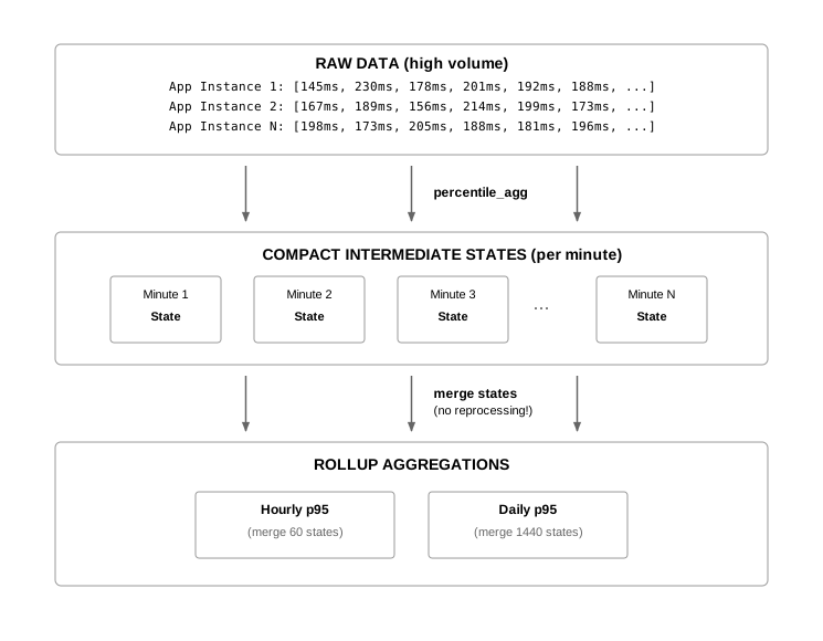The result? Scalable, real-time percentile analytics that deliver fast, accurate insights across high-ingest, high-resolution data, while keeping resource use lean.

includes all by default, while self-hosted includes a subset of them. For additional , install the extension.

For more information, read the blog post.

Common hyperfunction use cases

Learn how to use for specific analysis tasks:

• Analyse data distribution: use percentile approximation to understand data distribution in large datasets
• Count distinct values efficiently: use approximate count distinct to find the number of unique values, or cardinality, in a large dataset
• Monitor application performance: collect counter data with counter aggregation functions that handle resets and interruptions
• Gapfilling and interpolation: handle missing data when you query time-series data
• Analyze intermittent time-series data: analyze intermittent or irregular time-series data with heartbeat aggregation
• Calculate common statistical measures: use two-step aggregation for continuous aggregates and window functions
• Handle unevenly sampled time series data: use time-weighted averages and integrals with irregularly sampled time-series data

For a complete list of all , see the reference.

Function pipelines

Early access

Function pipelines are an experimental feature, designed to radically improve how you write queries to analyze data in and SQL. They work by applying principles from functional programming and popular tools like Python Pandas, and PromQL.

The timevector() function materializes all its data points in memory. This means that if you use it on a very large dataset, it runs out of memory. Do not use the timevector() function on a large dataset, or in production.

SQL is the best language for data analysis, but it is not perfect, and at times it can be difficult to construct the query you want. For example, this query gets data from the last day from the measurements table, sorts the data by the time column, calculates the delta between the values, takes the absolute value of the delta, and then takes the sum of the result of the previous steps:

SELECT device_id,
  sum(abs_delta) as volatility
FROM (
  SELECT device_id,
    abs(val - lag(val) OVER last_day) as abs_delta
  FROM measurements
  WHERE ts >= now()-'1 day'::interval
) calc_delta
GROUP BY device_id;

You can express the same query with a function pipeline like this:

SELECT device_id,
  toolkit_experimental.timevector(ts, val)
    -> toolkit_experimental.sort()
    -> toolkit_experimental.delta()
    -> toolkit_experimental.abs()
    -> toolkit_experimental.sum() as volatility
FROM measurements
WHERE ts >= now()-'1 day'::interval
GROUP BY device_id;

Function pipelines are completely SQL compliant, meaning that any tool that speaks SQL is able to support data analysis using function pipelines.

Anatomy of a function pipeline

Function pipelines are built as a series of elements that work together to create your query. The most important part of a pipeline is a custom data type called a timevector. The other elements then work on the timevector to build your query, using a custom operator to define the order in which the elements are run.

Timevectors

A timevector is a collection of time,value pairs with a defined start and end time, that could look something like this:

Your entire database might have time,value pairs that go well into the past and continue into the future, but the timevector has a defined start and end time within that dataset, which could look something like this:

To construct a timevector from your data, use a custom aggregate and pass in the columns to become the time,value pairs. It uses a WHERE clause to define the limits of the subset, and a GROUP BY clause to provide identifying information about the time-series. For example, to construct a timevector from a dataset that contains temperatures:

SELECT device_id,
  toolkit_experimental.timevector(ts, val)
FROM measurements
WHERE ts >= now() - '1 day'::interval
GROUP BY device_id;

Custom operator

Function pipelines use a single custom operator of ->. This operator is used to apply and compose multiple functions. The -> operator takes the inputs on the left of the operator, and applies the operation on the right of the operator. To put it more plainly, you can think of it as “do the next thing.”

A typical function pipeline could look something like this:

SELECT device_id,
  toolkit_experimental.timevector(ts, val)
    -> toolkit_experimental.sort()
    -> toolkit_experimental.delta()
    -> toolkit_experimental.abs()
    -> toolkit_experimental.sum() as volatility
FROM measurements
WHERE ts >= now() - '1 day'::interval
GROUP BY device_id;

While it might look at first glance as though timevector(ts, val) operation is an argument to sort(), in a pipeline these are all regular function calls. Each of the calls can only operate on the things in their own parentheses, and don’t know about anything to the left of them in the statement.

Each of the functions in a pipeline returns a custom type that describes the function and its arguments, these are all pipeline elements. The -> operator performs one of two different types of actions depending on the types on its right and left sides:

• Applies a pipeline element to the left hand argument: performing the function described by the pipeline element on the incoming data type directly.
• Compose pipeline elements into a combined element that can be applied at some point in the future. This is an optimization that allows you to nest elements to reduce the number of passes that are required.

The operator determines the action to perform based on its left and right arguments.

Pipeline elements

There are two main types of pipeline elements:

• Transforms change the contents of the timevector, returning the updated vector.
• Finalizers finish the pipeline and output the resulting data.

Transform elements take in a timevector and produce a timevector. They are the simplest element to compose, because they produce the same type. For example:

SELECT device_id,
  toolkit_experimental.timevector(ts, val)
    -> toolkit_experimental.sort()
    -> toolkit_experimental.delta()
    -> toolkit_experimental.map($$ ($value^3 + $value^2 + $value * 2) $$)
    -> toolkit_experimental.lttb(100)
FROM measurements

Finalizer elements end the timevector portion of a pipeline. They can produce an output in a specified format, or they can produce an aggregate of the timevector.

For example, a finalizer element that produces an output:

SELECT device_id,
  toolkit_experimental.timevector(ts, val)
    -> toolkit_experimental.sort()
    -> toolkit_experimental.delta()
    -> toolkit_experimental.unnest()
FROM measurements

Or a finalizer element that produces an aggregate:

SELECT device_id,
  toolkit_experimental.timevector(ts, val)
    -> toolkit_experimental.sort()
    -> toolkit_experimental.delta()
    -> toolkit_experimental.time_weight()
FROM measurements

The third type of pipeline elements are aggregate accessors and mutators. These work on a timevector in a pipeline, but they also work in regular aggregate queries. An example of using these in a pipeline:

SELECT percentile_agg(val) -> toolkit_experimental.approx_percentile(0.5)
FROM measurements

For a complete list of all pipeline elements, see the function pipeline elements reference.

For more information about how function pipelines work, read our blog post.