> ## Documentation Index
> Fetch the complete documentation index at: https://mintlify-poc.mintlify.site/llms.txt
> Use this file to discover all available pages before exploring further.
# Analyze Bitcoin blockchain
> Query and analyze blockchain transactions to discover insights about fees, mining revenue, and market trends
export const CLOUD_LONG = 'Tiger Cloud';
export const CAGG_CAP = 'Continuous aggregate';
export const CAGG = 'continuous aggregate';
export const CONSOLE = 'Tiger Console';
export const PG = 'Postgres';
export const HYPERTABLE_CAP = 'Hypertable';
export const HYPERCORE = 'hypercore';
export const ROWSTORE = 'rowstore';
export const HYPERCORE_CAP = 'Hypercore';
export const CHUNK = 'chunk';
export const HYPERTABLE = 'hypertable';
export const COLUMNSTORE = 'columnstore';
export const TIMESCALE_DB = 'TimescaleDB';
export const SERVICE_LONG = 'Tiger Cloud service';
export const SELF_LONG = 'self-hosted TimescaleDB';
export const SERVICE_SHORT = 'service';
export const COMPANY = 'Tiger Data ';
The financial industry is extremely data-heavy and relies on real-time and historical data for decision-making, risk assessment, fraud detection, and market analysis. {COMPANY} simplifies management of these large volumes of data, while also providing you with meaningful analytical insights and optimizing storage costs.
In this tutorial, you use {CLOUD_LONG} to ingest, store, and analyze transactions
on the Bitcoin blockchain.
[Blockchains][blockchain-def] are, at their essence, a distributed database. The
[transactions][transactions-def] in a blockchain are an example of time-series data. You can use
{TIMESCALE_DB} to query transactions on a blockchain, in exactly the same way as you
might query time-series transactions in any other database.
This tutorial uses a sample Bitcoin dataset and covers:
1. **Ingest data**: set up and connect to a {SERVICE_LONG}, create tables and {HYPERTABLE}s, and ingest data.
2. **Query the data**: obtain information about recent transactions and blocks using basic SQL queries.
3. **Analyze the data**: create {CAGG}s and use {TIMESCALE_DB} hyperfunctions to discover insights about transaction fees, mining revenue, and market correlations.
4. **Visualize results**: graph your analytical queries in Grafana dashboards.
## Prerequisites
To follow the steps on this page:
* Create a target [{SERVICE_LONG}][create-service] with Real-time analytics enabled.
You need [your connection details][connection-info]. This procedure also
works for [{SELF_LONG}][enable-timescaledb].
[create-service]: /deploy-and-operate/tiger-cloud/get-started/create-services
[enable-timescaledb]: /deploy-and-operate/self-hosted/install-and-update/install-self-hosted
[connection-info]: /integrations/find-connection-details
* Install and run [self-managed Grafana][grafana-self-managed], or sign up for [Grafana Cloud][grafana-cloud].
This tutorial uses a dataset that contains Bitcoin blockchain data for
the past five days, in a {HYPERTABLE} named `transactions`.
## Optimize time-series data using hypertables
{HYPERTABLE_CAP}s are {PG} tables in {TIMESCALE_DB} that automatically partition your time-series data by time. Time-series data represents the way a system, process, or behavior changes over time. {HYPERTABLE_CAP}s enable {TIMESCALE_DB} to work efficiently with time-series data. Each {HYPERTABLE} is made up of child tables called chunks. Each chunk is assigned a range of time, and only contains data from that range. When you run a query, {TIMESCALE_DB} identifies the correct chunk and runs the query on it, instead of going through the entire table.
[{HYPERCORE_CAP}][hypercore] is the hybrid row-columnar storage engine in {TIMESCALE_DB} used by {HYPERTABLE}s. Traditional
databases force a trade-off between fast inserts (row-based storage) and efficient analytics
(columnar storage). {HYPERCORE_CAP} eliminates this trade-off, allowing real-time analytics without sacrificing
transactional capabilities.
{HYPERCORE_CAP} dynamically stores data in the most efficient format for its lifecycle:
![Move from rowstore to columstore in hypercore][move-from-rowstore-to-columstore-in-hypercore]
* **Row-based storage for recent data**: the most recent chunk (and possibly more) is always stored in the {ROWSTORE},
ensuring fast inserts, updates, and low-latency single record queries. Additionally, row-based storage is used as a
writethrough for inserts and updates to columnar storage.
* **Columnar storage for analytical performance**: chunks are automatically compressed into the {COLUMNSTORE}, optimizing
storage efficiency and accelerating analytical queries.
Unlike traditional columnar databases, {HYPERCORE} allows data to be inserted or modified at any stage, making it a
flexible solution for both high-ingest transactional workloads and real-time analytics—within a single database.
[hypercore]: /manage-data/capabilities/hypercore/understand-hypercore
[move-from-rowstore-to-columstore-in-hypercore]: https://assets.timescale.com/docs/images/hypercore_intro.svg
Because {TIMESCALE_DB} is 100% {PG}, you can use all the standard {PG} tables, indexes, stored procedures, and other objects alongside your {HYPERTABLE}s. This makes creating and working with {HYPERTABLE}s similar to standard {PG}.
1. Connect to your {SERVICE_LONG}
In [{CONSOLE}][services-portal] open an [SQL editor][in-console-editors]. The in-Console editors display the query speed.
You can also connect to your service using [psql][connect-using-psql].
2. Create a [{HYPERTABLE}][hypertables-section] for your time-series data using [CREATE TABLE][hypertable-create-table].
For [efficient queries][secondary-indexes] on data in the {COLUMNSTORE}, remember to `segmentby` the column you will
use most often to filter your data:
```sql theme={"dark"}
CREATE TABLE transactions (
time TIMESTAMPTZ NOT NULL,
block_id INT,
hash TEXT,
size INT,
weight INT,
is_coinbase BOOLEAN,
output_total BIGINT,
output_total_usd DOUBLE PRECISION,
fee BIGINT,
fee_usd DOUBLE PRECISION,
details JSONB
) WITH (
tsdb.hypertable,
tsdb.segmentby='block_id',
tsdb.orderby='time DESC'
);
```
When you create a {HYPERTABLE} using [CREATE TABLE ... WITH ...][hypertable-create-table], the default partitioning
column is automatically the first column with a timestamp data type. Also, {TIMESCALE_DB} creates a
[columnstore policy][add_columnstore_policy] that automatically converts your data to the {COLUMNSTORE}, after an
interval equal to the value of the [chunk\_interval][create_table_arguments], defined through `compress_after` in the
policy. This columnar format enables fast scanning and
aggregation, optimizing performance for analytical workloads while also saving significant storage space. In the
{COLUMNSTORE} conversion, {HYPERTABLE} {CHUNK}s are compressed by up to 98%, and organized for efficient, large-scale queries.
You can customize this policy later using [alter\_job][alter_job_samples]. However, to change `after` or
`created_before`, the compression settings, or the {HYPERTABLE} the policy is acting on, you must
[remove the columnstore policy][remove_columnstore_policy] and [add a new one][add_columnstore_policy].
You can also manually [convert {CHUNK}s][convert_to_columnstore] in a {HYPERTABLE} to the {COLUMNSTORE}.
[add_columnstore_policy]: /api-reference/timescaledb/hypercore/add_columnstore_policy
[alter_job_samples]: /api-reference/timescaledb/jobs-automation/alter_job#samples
[convert_to_columnstore]: /api-reference/timescaledb/hypercore/convert_to_columnstore
[create_table_arguments]: /api-reference/timescaledb/hypertables/create_table#arguments
[hypertable-create-table]: /api-reference/timescaledb/hypertables/create_table
[remove_columnstore_policy]: /api-reference/timescaledb/hypercore/remove_columnstore_policy
3. Create an index on the `hash` column to make queries for individual
transactions faster:
```sql theme={"dark"}
CREATE INDEX hash_idx ON public.transactions USING HASH (hash);
```
4. Create an index on the `block_id` column to make block-level queries faster:
When you create a {HYPERTABLE}, it is partitioned on the time column. {TIMESCALE_DB}
automatically creates an index on the time column. However, you'll often filter
your time-series data on other columns as well. You use [indexes][indexing] to improve
query performance.
```sql theme={"dark"}
CREATE INDEX block_idx ON public.transactions (block_id);
```
5. Create a unique index on the `time` and `hash` columns to make sure you
don't accidentally insert duplicate records:
```sql theme={"dark"}
CREATE UNIQUE INDEX time_hash_idx ON public.transactions (time, hash);
```
[connect-using-psql]: /integrations/psql#connect-to-your-service
[hypertable-create-table]: /api-reference/timescaledb/hypertables/create_table
[hypertables-section]: /manage-data/data-management/hypertables/understand-hypertables
[in-console-editors]: /deploy-and-operate/tiger-cloud/get-started/run-queries-from-console
[indexing]: /manage-data/data-management/indexing
[secondary-indexes]: /use-timescale/hypercore/secondary-indexes
[services-portal]: https://console.cloud.timescale.com/dashboard/services
## Load financial data
The dataset contains around 1.5 million Bitcoin transactions, the trades for five days. It includes
information about each transaction, along with the value in [satoshi][satoshi-def]. It also states if a
trade is a [coinbase][coinbase-def] transaction, and the reward a coin miner receives for mining the coin.
To ingest data into the tables that you created, you need to download the
dataset and copy the data to your database.
1. Download the `bitcoin_sample.zip` file. The file contains a `.csv`
file that contains Bitcoin transactions for the past five days:
[bitcoin\_sample.zip][bitcoin_samplezip]
2. In a new terminal window, run this command to unzip the `.csv` files:
```bash theme={"dark"}
unzip bitcoin_sample.zip
```
3. In Terminal, navigate to the folder where you unzipped the Bitcoin transactions, then
connect to your {SERVICE_SHORT} using [psql][connect-using-psql].
4. At the `psql` prompt, use the `COPY` command to transfer data into your
{SERVICE_LONG}. If the `.csv` files aren't in your current directory,
specify the file paths in these commands:
```sql theme={"dark"}
\COPY transactions FROM 'tutorial_bitcoin_sample.csv' CSV HEADER;
```
Because there is over a million rows of data, the `COPY` process could take
a few minutes depending on your internet connection and local client
resources.
[bitcoin_samplezip]: https://assets.timescale.com/docs/downloads/bitcoin-blockchain/bitcoin_sample.zip
[coinbase-def]: https://www.pcmag.com/encyclopedia/term/coinbase-transaction
[connect-using-psql]: /integrations/psql#connect-to-your-service
[satoshi-def]: https://www.pcmag.com/encyclopedia/term/satoshi
## Connect Grafana to Tiger Cloud
To visualize the results of your queries, enable Grafana to read the data in your {SERVICE_SHORT}:
1. **Log in to Grafana**
In your browser, log in to either:
* Self-hosted Grafana: at `http://localhost:3000/`. The default credentials are `admin`, `admin`.
* Grafana Cloud: use the URL and credentials you set when you created your account.
2. **Add your {SERVICE_SHORT} as a data source**
1. Open `Connections` > `Data sources`, then click `Add new data source`.
2. Select `PostgreSQL` from the list.
3. Configure the connection:
* `Host URL`, `Database name`, `Username`, and `Password`
Configure using your [connection details][connection-info]. `Host URL` is in the format `:`.
* `TLS/SSL Mode`: select `require`.
* `PostgreSQL options`: enable `TimescaleDB`.
* Leave the default setting for all other fields.
4. Click `Save & test`.
Grafana checks that your details are set correctly.
[cloud-login]: https://console.cloud.timescale.com/
[connection-info]: /integrations/find-connection-details
[create-service]: /deploy-and-operate/tiger-cloud/get-started/create-services
[grafana-cloud]: https://grafana.com/get/
[grafana-self-managed]: https://grafana.com/get/?tab=self-managed
## Query the data
When you have your dataset loaded, you can start constructing some queries to
discover what your data tells you. In this section, you learn how to write
queries that answer these questions:
* [What are the five most recent coinbase transactions?](#what-are-the-five-most-recent-coinbase-transactions)
* [What are the five most recent transactions?](#what-are-the-five-most-recent-transactions)
* [What are the five most recent blocks?](#what-are-the-five-most-recent-blocks)
### What are the five most recent coinbase transactions?
[Coinbase][coinbase-def] transactions are the first transaction in a block, and
they include the reward a coin miner receives for mining the coin. To find the
most recent coinbase transactions, you can query for transactions where
`is_coinbase` is TRUE. You'll notice that the `fee_usd` is \$0 for each coinbase
transaction because the miner receives the block reward directly without paying
a transaction fee.
1. Connect to the {SERVICE_LONG} that contains the Bitcoin dataset.
2. At the psql prompt, use this query to select the five most recent
coinbase transactions:
```sql theme={"dark"}
SELECT time, hash, block_id, fee_usd FROM transactions
WHERE is_coinbase IS TRUE
ORDER BY time DESC
LIMIT 5;
```
3. The data you get back looks a bit like this:
```sql theme={"dark"}
time | hash | block_id | fee_usd
------------------------+------------------------------------------------------------------+----------+---------
2023-06-12 23:54:18+00 | 22e4610bc12d482bc49b7a1c5b27ad18df1a6f34256c16ee7e499b511e02d71e | 794111 | 0
2023-06-12 23:53:08+00 | dde958bb96a302fd956ced32d7b98dd9860ff82d569163968ecfe29de457fedb | 794110 | 0
2023-06-12 23:44:50+00 | 75ac1fa7febe1233ee57ca11180124c5ceb61b230cdbcbcba99aecc6a3e2a868 | 794109 | 0
2023-06-12 23:44:14+00 | 1e941d66b92bf0384514ecb83231854246a94c86ff26270fbdd9bc396dbcdb7b | 794108 | 0
2023-06-12 23:41:08+00 | 60ae50447254d5f4561e1c297ee8171bb999b6310d519a0d228786b36c9ffacf | 794107 | 0
(5 rows)
```
### What are the five most recent transactions?
This dataset contains Bitcoin transactions for the last five days. To find out
the most recent transactions in the dataset, you can use a `SELECT` statement.
In this case, you want to find transactions that are not coinbase transactions,
sort them by time in descending order, and take the top five results. You also
want to see the block ID, and the value of the transaction in US Dollars.
1. Connect to the {SERVICE_LONG} that contains the Bitcoin dataset.
2. At the psql prompt, use this query to select the five most recent
non-coinbase transactions:
```sql theme={"dark"}
SELECT time, hash, block_id, fee_usd FROM transactions
WHERE is_coinbase IS NOT TRUE
ORDER BY time DESC
LIMIT 5;
```
3. The data you get back looks a bit like this:
```sql theme={"dark"}
time | hash | block_id | fee_usd
------------------------+------------------------------------------------------------------+----------+---------
2023-06-12 23:54:18+00 | 6f709d52e9aa7b2569a7f8c40e7686026ede6190d0532220a73fdac09deff973 | 794111 | 7.614
2023-06-12 23:54:18+00 | ece5429f4a76b1603aecbee31bf3d05f74142a260e4023316250849fe49115ae | 794111 | 9.306
2023-06-12 23:54:18+00 | 54a196398880a7e2e38312d4285fa66b9c7129f7d14dc68c715d783322544942 | 794111 | 13.1928
2023-06-12 23:54:18+00 | 3e83e68735af556d9385427183e8160516fafe2f30f30405711c4d64bf0778a6 | 794111 | 3.5416
2023-06-12 23:54:18+00 | ca20d073b1082d7700b3706fe2c20bc488d2fc4a9bb006eb4449efe3c3fc6b2b | 794111 | 8.6842
(5 rows)
```
### What are the five most recent blocks?
In this procedure, you use a more complicated query to return the five most
recent blocks, and show some additional information about each, including the
block weight, number of transactions in each block, and the total block value in
US Dollars.
1. Connect to the {SERVICE_LONG} that contains the Bitcoin dataset.
2. At the psql prompt, use this query to select the five most recent
blocks:
```sql theme={"dark"}
WITH recent_blocks AS (
SELECT block_id FROM transactions
WHERE is_coinbase IS TRUE
ORDER BY time DESC
LIMIT 5
)
SELECT
t.block_id, count(*) AS transaction_count,
SUM(weight) AS block_weight,
SUM(output_total_usd) AS block_value_usd
FROM transactions t
INNER JOIN recent_blocks b ON b.block_id = t.block_id
WHERE is_coinbase IS NOT TRUE
GROUP BY t.block_id;
```
3. The data you get back looks a bit like this:
```sql theme={"dark"}
block_id | transaction_count | block_weight | block_value_usd
----------+-------------------+--------------+--------------------
794108 | 5625 | 3991408 | 65222453.36381342
794111 | 5039 | 3991748 | 5966031.481099684
794109 | 6325 | 3991923 | 5406755.801599815
794110 | 2525 | 3995553 | 177249139.6457974
794107 | 4464 | 3991838 | 107348519.36559173
(5 rows)
```
## Analyze the data
In this section, you use [{TIMESCALE_DB} hyperfunctions][understand-hyperfunctions] to construct
analytical queries that are not possible in standard {PG}. You create {CAGG}s
to simplify and speed up your queries, then use them to answer these questions:
* Is there any connection between the number of transactions and the transaction fees?
* Does the transaction volume affect the BTC-USD rate?
* Do more transactions in a block mean the block is more expensive to mine?
* What percentage of the average miner's revenue comes from fees compared to block rewards?
* How does block weight affect miner fees?
* What's the average miner revenue per block?
### Create continuous aggregates
You can use [{CAGG}s][docs-cagg] to simplify and speed up your
queries. For this analysis, you need three {CAGG}s focusing on
three aspects of the dataset: Bitcoin transactions, blocks, and coinbase
transactions. In each {CAGG} definition, the `time_bucket()`
function controls how large the time buckets are. The examples all use 1-hour
time buckets.
1. Connect to the {SERVICE_LONG} that contains the Bitcoin dataset.
2. Create a {CAGG} called
`one_hour_transactions`. This view holds aggregated data about each hour of
transactions:
```sql theme={"dark"}
CREATE MATERIALIZED VIEW one_hour_transactions
WITH (timescaledb.continuous) AS
SELECT time_bucket('1 hour', time) AS bucket,
count(*) AS tx_count,
sum(fee) AS total_fee_sat,
sum(fee_usd) AS total_fee_usd,
stats_agg(fee) AS stats_fee_sat,
avg(size) AS avg_tx_size,
avg(weight) AS avg_tx_weight,
count(
CASE
WHEN (fee > output_total) THEN hash
ELSE NULL
END) AS high_fee_count
FROM transactions
WHERE (is_coinbase IS NOT TRUE)
GROUP BY bucket;
```
3. Add a refresh policy to keep the {CAGG} up-to-date:
```sql theme={"dark"}
SELECT add_continuous_aggregate_policy('one_hour_transactions',
start_offset => INTERVAL '3 hours',
end_offset => INTERVAL '1 hour',
schedule_interval => INTERVAL '1 hour');
```
4. Create a {CAGG} called `one_hour_blocks`. This view holds
aggregated data about all the blocks that were mined each hour:
```sql theme={"dark"}
CREATE MATERIALIZED VIEW one_hour_blocks
WITH (timescaledb.continuous) AS
SELECT time_bucket('1 hour', time) AS bucket,
block_id,
count(*) AS tx_count,
sum(fee) AS block_fee_sat,
sum(fee_usd) AS block_fee_usd,
stats_agg(fee) AS stats_tx_fee_sat,
avg(size) AS avg_tx_size,
avg(weight) AS avg_tx_weight,
sum(size) AS block_size,
sum(weight) AS block_weight,
max(size) AS max_tx_size,
max(weight) AS max_tx_weight,
min(size) AS min_tx_size,
min(weight) AS min_tx_weight
FROM transactions
WHERE is_coinbase IS NOT TRUE
GROUP BY bucket, block_id;
```
5. Add a refresh policy to keep the {CAGG} up to date:
```sql theme={"dark"}
SELECT add_continuous_aggregate_policy('one_hour_blocks',
start_offset => INTERVAL '3 hours',
end_offset => INTERVAL '1 hour',
schedule_interval => INTERVAL '1 hour');
```
6. Create a {CAGG} called `one_hour_coinbase`. This view holds
aggregated data about all the transactions that miners received as rewards
each hour:
```sql theme={"dark"}
CREATE MATERIALIZED VIEW one_hour_coinbase
WITH (timescaledb.continuous) AS
SELECT time_bucket('1 hour', time) AS bucket,
count(*) AS tx_count,
stats_agg(output_total, output_total_usd) AS stats_miner_revenue,
min(output_total) AS min_miner_revenue,
max(output_total) AS max_miner_revenue
FROM transactions
WHERE is_coinbase IS TRUE
GROUP BY bucket;
```
7. Add a refresh policy to keep the {CAGG} up to date:
```sql theme={"dark"}
SELECT add_continuous_aggregate_policy('one_hour_coinbase',
start_offset => INTERVAL '3 hours',
end_offset => INTERVAL '1 hour',
schedule_interval => INTERVAL '1 hour');
```
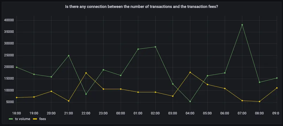
### Is there any connection between the number of transactions and the transaction fees?
Transaction fees are a major concern for blockchain users. If a blockchain is
too expensive, you might not want to use it. This query shows you whether
there's any correlation between the number of Bitcoin transactions and the fees.
The time range for this analysis is the last 2 days.
If you choose to visualize the query in Grafana, you can see the average
transaction volume and the average fee per transaction, over time. These trends
might help you decide whether to submit a transaction now or wait a few days for
fees to decrease.
1. Connect to the {SERVICE_LONG} that contains the Bitcoin dataset.
2. At the psql prompt, use this query to average transaction volume and the
fees from the `one_hour_transactions` {CAGG}:
```sql theme={"dark"}
SELECT
bucket AS "time",
tx_count as "tx volume",
average(stats_fee_sat) as fees
FROM one_hour_transactions
WHERE bucket > date_add('2023-11-22 00:00:00+00', INTERVAL '-2 days')
ORDER BY 1;
```
3. The data you get back looks a bit like this:
```sql theme={"dark"}
time | tx volume | fees
------------------------+-----------+--------------------
2023-11-20 01:00:00+00 | 2602 | 105963.45810914681
2023-11-20 02:00:00+00 | 33037 | 26686.814117504615
2023-11-20 03:00:00+00 | 42077 | 22875.286546094067
2023-11-20 04:00:00+00 | 46021 | 20280.843180287262
2023-11-20 05:00:00+00 | 20828 | 24694.472969080085
...
```
4. To visualize this in Grafana:
1. From the `Dashboards` page, click `New` and select `New dashboard`.
2. Click `Add visualization`, then select the data source that connects to your {SERVICE_LONG}.
3. In the `Queries` section, change the `Format` to `Time series` and select `Code`.
4. Type the query from the previous step and click `Run query`.
### Does the transaction volume affect the BTC-USD rate?
In cryptocurrency trading, there's a lot of speculation. You can adopt a
data-based trading strategy by looking at correlations between blockchain
metrics, such as transaction volume and the current exchange rate between
Bitcoin and US Dollars.
If you choose to visualize the query in Grafana, you can see the average
transaction volume, along with the BTC to US Dollar conversion rate.
1. Connect to the {SERVICE_LONG} that contains the Bitcoin dataset.
2. At the psql prompt, use this query to return the trading volume and the BTC
to US Dollar exchange rate:
```sql theme={"dark"}
SELECT
bucket AS "time",
tx_count as "tx volume",
total_fee_usd / (total_fee_sat*0.00000001) AS "btc-usd rate"
FROM one_hour_transactions
WHERE bucket > date_add('2023-11-22 00:00:00+00', INTERVAL '-2 days')
ORDER BY 1;
```
3. The data you get back looks a bit like this:
```sql theme={"dark"}
time | tx volume | btc-usd rate
------------------------+-----------+--------------------
2023-06-13 08:00:00+00 | 20063 | 25975.888587931426
2023-06-13 09:00:00+00 | 16984 | 25976.00446352126
2023-06-13 10:00:00+00 | 15856 | 25975.988587014584
2023-06-13 11:00:00+00 | 24967 | 25975.89166787936
2023-06-13 12:00:00+00 | 8575 | 25976.004209699528
...
```
4. To visualize this in Grafana:
1. From the `Dashboards` page, click `New` and select `New dashboard`.
2. Click `Add visualization`, then select the data source that connects to your {SERVICE_LONG}.
3. In the `Queries` section, change the `Format` to `Time series` and select `Code`.
4. Type the query from the previous step and click `Run query`.
5. Under the panel options on the right, click `Add field override` > `Fields with name`, then choose `btc-usd rate` in the dropdown.
6. Click `Add override property`, then select `Axis > Placement` and click `Right`.

### Do more transactions in a block mean the block is more expensive to mine?
The number of transactions in a block can influence the overall block mining
fee. For this analysis, a larger time frame is required, so increase the
analyzed time range to 5 days.
If you choose to visualize the query in Grafana, you can see that the more
transactions in a block, the higher the mining fee becomes.
1. Connect to the {SERVICE_LONG} that contains the Bitcoin dataset.
2. At the psql prompt, use this query to return the number of transactions in a
block, compared to the mining fee:
```sql theme={"dark"}
SELECT
bucket as "time",
avg(tx_count) AS transactions,
avg(block_fee_sat)*0.00000001 AS "mining fee"
FROM one_hour_blocks
WHERE bucket > date_add('2023-11-22 00:00:00+00', INTERVAL '-5 days')
GROUP BY bucket
ORDER BY 1;
```
3. The data you get back looks a bit like this:
```sql theme={"dark"}
time | transactions | mining fee
------------------------+-----------------------+------------------------
2023-06-10 08:00:00+00 | 2322.2500000000000000 | 0.29221418750000000000
2023-06-10 09:00:00+00 | 3305.0000000000000000 | 0.50512649666666666667
2023-06-10 10:00:00+00 | 3011.7500000000000000 | 0.44783255750000000000
2023-06-10 11:00:00+00 | 2874.7500000000000000 | 0.39303009500000000000
2023-06-10 12:00:00+00 | 2339.5714285714285714 | 0.25590717142857142857
```
4. To visualize this in Grafana:
1. From the `Dashboards` page, click `New` and select `New dashboard`.
2. Click `Add visualization`, then select the data source that connects to your {SERVICE_LONG}.
3. In the `Queries` section, change the `Format` to `Time series` and select `Code`.
4. Type the query from the previous step and click `Run query`.
5. Under the panel options on the right, click `Add field override` > `Fields with name`, then choose `mining fee` in the dropdown.
6. Click `Add override property`, then select `Axis > Placement` and click `Right`.

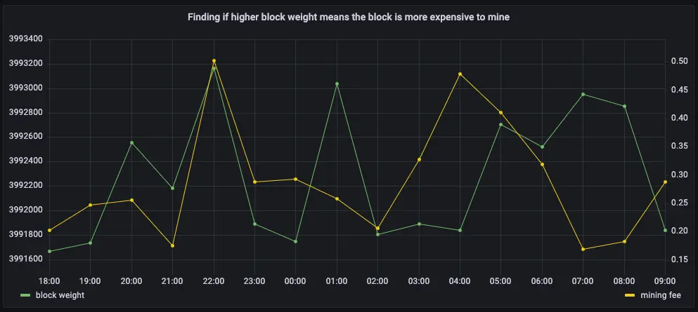
You can extend this analysis to find if there is the same correlation between
block weight and mining fee. More transactions should increase the block weight,
and boost the miner fee as well.
If you choose to visualize the query in Grafana, you can see the same kind of
high correlation between block weight and mining fee. The relationship weakens
when the block weight gets close to its maximum value, which is 4 million weight
units, in which case it's impossible for a block to include more transactions.
1. Connect to the {SERVICE_LONG} that contains the Bitcoin dataset.
2. At the psql prompt, use this query to return the block weight, compared to
the mining fee:
```sql theme={"dark"}
SELECT
bucket as "time",
avg(block_weight) as "block weight",
avg(block_fee_sat*0.00000001) as "mining fee"
FROM one_hour_blocks
WHERE bucket > date_add('2023-11-22 00:00:00+00', INTERVAL '-5 days')
group by bucket
ORDER BY 1;
```
3. The data you get back looks a bit like this:
```sql theme={"dark"}
time | block weight | mining fee
------------------------+----------------------+------------------------
2023-06-10 08:00:00+00 | 3992809.250000000000 | 0.29221418750000000000
2023-06-10 09:00:00+00 | 3991766.333333333333 | 0.50512649666666666667
2023-06-10 10:00:00+00 | 3992918.250000000000 | 0.44783255750000000000
2023-06-10 11:00:00+00 | 3991873.000000000000 | 0.39303009500000000000
2023-06-10 12:00:00+00 | 3992934.000000000000 | 0.25590717142857142857
...
```
4. To visualize this in Grafana:
1. From the `Dashboards` page, click `New` and select `New dashboard`.
2. Click `Add visualization`, then select the data source that connects to your {SERVICE_LONG}.
3. In the `Queries` section, change the `Format` to `Time series` and select `Code`.
4. Type the query from the previous step and click `Run query`.
5. Under the panel options on the right, click `Add field override` > `Fields with name`, then choose `mining fee` in the dropdown.
6. Click `Add override property`, then select `Axis > Placement` and click `Right`.
### What percentage of the average miner's revenue comes from fees compared to block rewards?
In the previous queries, you saw that mining fees are higher when block weights
and transaction volumes are higher. This query analyzes the data from a
different perspective. Miner revenue is not only made up of miner fees, it also
includes block rewards for mining a new block. This reward is currently 6.25
BTC, and it gets halved every four years. This query looks at how much of a
miner's revenue comes from fees, compares to block rewards.
If you choose to visualize the query in Grafana, you can see that most miner
revenue actually comes from block rewards. Fees never account for more than a
few percentage points of overall revenue.
1. Connect to the {SERVICE_LONG} that contains the Bitcoin dataset.
2. At the psql prompt, use this query to return coinbase transactions, along
with the block fees and rewards:
```sql theme={"dark"}
WITH coinbase AS (
SELECT block_id, output_total AS coinbase_tx FROM transactions
WHERE is_coinbase IS TRUE and time > date_add('2023-11-22 00:00:00+00', INTERVAL '-5 days')
)
SELECT
bucket as "time",
avg(block_fee_sat)*0.00000001 AS "fees",
FIRST((c.coinbase_tx - block_fee_sat), bucket)*0.00000001 AS "reward"
FROM one_hour_blocks b
INNER JOIN coinbase c ON c.block_id = b.block_id
GROUP BY bucket
ORDER BY 1;
```
3. The data you get back looks a bit like this:
```sql theme={"dark"}
time | fees | reward
------------------------+------------------------+------------
2023-06-10 08:00:00+00 | 0.28247062857142857143 | 6.25000000
2023-06-10 09:00:00+00 | 0.50512649666666666667 | 6.25000000
2023-06-10 10:00:00+00 | 0.44783255750000000000 | 6.25000000
2023-06-10 11:00:00+00 | 0.39303009500000000000 | 6.25000000
2023-06-10 12:00:00+00 | 0.25590717142857142857 | 6.25000000
...
```
4. To visualize this in Grafana:
1. From the `Dashboards` page, click `New` and select `New dashboard`.
2. Click `Add visualization`, then select the data source that connects to your {SERVICE_LONG}.
3. In the `Queries` section, change the `Format` to `Time series` and select `Code`.
4. Type the query from the previous step and click `Run query`.
5. In the options panel, in the `Graph styles` section, for `Stack series` select `100%`.

### How does block weight affect miner fees?
You've already found that more transactions in a block mean it's more expensive
to mine. In this query, you ask if the same is true for block weights? The more
transactions a block has, the larger its weight, so the block weight and mining
fee should be tightly correlated. This query uses a 12-hour moving average to
calculate the block weight and block mining fee over time.
If you choose to visualize the query in Grafana, you can see that the block
weight and block mining fee are tightly connected. In practice, you can also see
the four million weight units size limit. This means that there's still room to
grow for individual blocks, and they could include even more transactions.
1. Connect to the {SERVICE_LONG} that contains the Bitcoin dataset.
2. At the psql prompt, use this query to return block weight, along with the
block fees and rewards:
```sql theme={"dark"}
WITH stats AS (
SELECT
bucket,
stats_agg(block_weight, block_fee_sat) AS block_stats
FROM one_hour_blocks
WHERE bucket > date_add('2023-11-22 00:00:00+00', INTERVAL '-5 days')
GROUP BY bucket
)
SELECT
bucket as "time",
average_y(rolling(block_stats) OVER (ORDER BY bucket RANGE '12 hours' PRECEDING)) AS "block weight",
average_x(rolling(block_stats) OVER (ORDER BY bucket RANGE '12 hours' PRECEDING))*0.00000001 AS "mining fee"
FROM stats
ORDER BY 1;
```
3. The data you get back looks a bit like this:
```sql theme={"dark"}
time | block weight | mining fee
------------------------+--------------------+---------------------
2023-06-10 09:00:00+00 | 3991766.3333333335 | 0.5051264966666666
2023-06-10 10:00:00+00 | 3992424.5714285714 | 0.47238710285714286
2023-06-10 11:00:00+00 | 3992224 | 0.44353000909090906
2023-06-10 12:00:00+00 | 3992500.111111111 | 0.37056557222222225
2023-06-10 13:00:00+00 | 3992446.65 | 0.39728022799999996
...
```
4. To visualize this in Grafana:
1. From the `Dashboards` page, click `New` and select `New dashboard`.
2. Click `Add visualization`, then select the data source that connects to your {SERVICE_LONG}.
3. In the `Queries` section, change the `Format` to `Time series` and select `Code`.
4. Type the query from the previous step and click `Run query`.
5. Under the panel options on the right, click `Add field override` > `Fields with name`, then choose `mining fee` in the dropdown.
6. Click `Add override property`, then select `Axis > Placement` and click `Right`.

### What's the average miner revenue per block?
In this final query, you analyze how much revenue miners actually generate by
mining a new block on the blockchain, including fees and block rewards. To make
the analysis more interesting, add the Bitcoin to US Dollar exchange rate, and
increase the time range.
1. Connect to the {SERVICE_LONG} that contains the Bitcoin dataset.
2. At the psql prompt, use this query to return the average miner revenue per
block, with a 12-hour moving average:
```sql theme={"dark"}
SELECT
bucket as "time",
average_y(rolling(stats_miner_revenue) OVER (ORDER BY bucket RANGE '12 hours' PRECEDING))*0.00000001 AS "revenue in BTC",
average_x(rolling(stats_miner_revenue) OVER (ORDER BY bucket RANGE '12 hours' PRECEDING)) AS "revenue in USD"
FROM one_hour_coinbase
WHERE bucket > date_add('2023-11-22 00:00:00+00', INTERVAL '-5 days')
ORDER BY 1;
```
3. The data you get back looks a bit like this:
```sql theme={"dark"}
time | revenue in BTC | revenue in USD
------------------------+--------------------+--------------------
2023-06-09 14:00:00+00 | 6.6732841925 | 176922.1133
2023-06-09 15:00:00+00 | 6.785046736363636 | 179885.1576818182
2023-06-09 16:00:00+00 | 6.7252952905 | 178301.02735000002
2023-06-09 17:00:00+00 | 6.716377454814815 | 178064.5978074074
2023-06-09 18:00:00+00 | 6.7784206471875 | 179709.487309375
...
```
4. To visualize this in Grafana:
1. From the `Dashboards` page, click `New` and select `New dashboard`.
2. Click `Add visualization`, then select the data source that connects to your {SERVICE_LONG}.
3. In the `Queries` section, change the `Format` to `Time series` and select `Code`.
4. Type the query from the previous step and click `Run query`.
5. Under the panel options on the right, click `Add field override` > `Fields with name`, then choose `revenue in USD` in the dropdown.
6. Click `Add override property`, then select `Axis > Placement` and click `Right`.

[understand-hyperfunctions]: /api-reference/timescaledb/hyperfunctions/
[blockchain-def]: https://www.pcmag.com/encyclopedia/term/blockchain
[coinbase-def]: https://www.pcmag.com/encyclopedia/term/coinbase-transaction
[docs-cagg]: /manage-data/data-management/continuous-aggregates/understand-continuous-aggregates
[grafana-cloud]: https://grafana.com/get/
[grafana-self-managed]: https://grafana.com/get/?tab=self-managed
[transactions-def]: https://www.pcmag.com/encyclopedia/term/bitcoin-transaction