Aggregate data by time interval

Group hypertable data into time intervals using time_bucket. Calculate sums, averages, and aggregates over seconds, minutes, hours, or days

The time_bucket function enables you to aggregate data in a hypertable into buckets of time. For example, 5 minutes, 1 hour, or 3 days. time_bucket is similar to ‘s date_bin function, but it gives you more flexibility in the bucket size and start time.

You can use time_bucket to roll up data for analysis or downsampling. For example, you can calculate 5-minute averages for a sensor reading over the last day. You can perform these rollups as needed, or pre-calculate them in continuous aggregates.

How time bucketing works

Time bucketing groups data into time intervals. With time_bucket, the interval length can be any number of microseconds, milliseconds, seconds, minutes, hours, days, weeks, months, years, or centuries.

The time_bucket function is usually used in combination with GROUP BY to aggregate data. For example, you can calculate the average, maximum, minimum, or sum of values within a bucket.

Origin

The origin determines when time buckets start and end. By default, a time bucket doesn’t start at the earliest timestamp in your data. There is often a more logical time. For example, you might collect your first data point at 00:37, but you probably want your daily buckets to start at midnight. Similarly, you might collect your first data point on a Wednesday, but you might want your weekly buckets calculated from Sunday or Monday.

Instead, time is divided into buckets based on intervals from the origin. The following diagram shows how, using the example of 2-week buckets. The first possible start date for a bucket is origin. The next possible start date for a bucket is origin + bucket interval. If your first timestamp does not fall exactly on a possible start date, the immediately preceding start date is used for the beginning of the bucket.

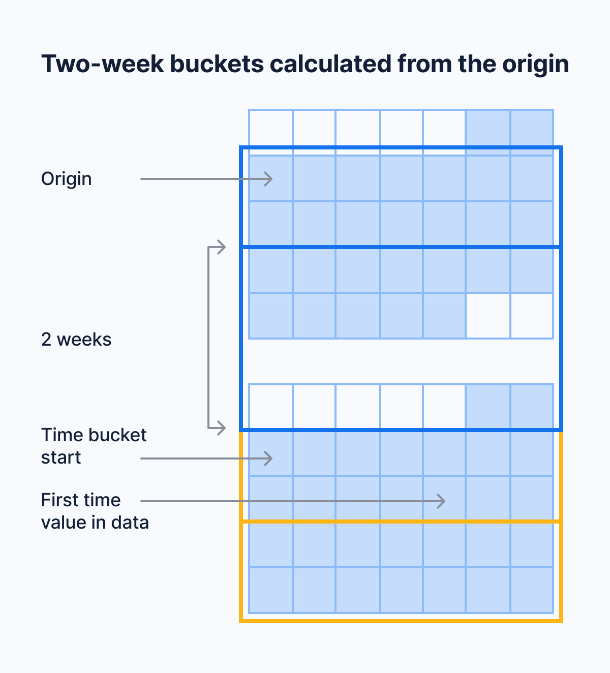For example, say that your data’s earliest timestamp is April 24, 2020. If you bucket by an interval of two weeks, the first bucket doesn’t start on April 24, which is a Friday. It also doesn’t start on April 20, which is the immediately precedisng Monday. It starts on April 13, because you can get to April 13, 2020, by counting in two-week increments from January 3, 2000, which is the default origin in this case.

Default origins

For intervals that don’t include months or years, the default origin is January 3, 2000. For month, year, or century intervals, the default origin is January 1, 2000. For integer time values, the default origin is 0.

These choices make the time ranges of time buckets more intuitive. Because January 3, 2000, is a Monday, weekly time buckets start on Monday. This is compliant with the ISO standard for calculating calendar weeks. Monthly and yearly time buckets use January 1, 2000, as an origin. This allows them to start on the first day of the calendar month or year.

If you prefer another origin, you can set it yourself using the origin parameter. For example, to start weeks on Sunday, set the origin to Sunday, January 2, 2000.

Timezones

The origin time depends on the data type of your time values.

If you use TIMESTAMP, by default, bucket start times are aligned with 00:00:00. Daily and weekly buckets start at 00:00:00. Shorter buckets start at a time that you can get to by counting in bucket increments from 00:00:00 on the origin date.

If you use TIMESTAMPTZ, by default, bucket start times are aligned with 00:00:00 UTC. To align time buckets to another timezone, set the timezone parameter.

Aggregate time-series data with time_bucket

The time_bucket function helps you group data in a hypertable so you can perform aggregate calculations over arbitrary time intervals. It is usually used in combination with GROUP BY for this purpose.

Group data by time buckets and calculate a summary value

Group data into time buckets and calculate a summary value for a column. For example, calculate the average daily temperature in a table named weather_conditions. The table has a time column named time and a temperature column:

SELECT time_bucket('1 day', time) AS bucket,
  avg(temperature) AS avg_temp
FROM weather_conditions
GROUP BY bucket
ORDER BY bucket ASC;

The time_bucket function returns the start time of the bucket. In this example, the first bucket starts at midnight on November 15, 2016, and aggregates all the data from that day:

bucket                 |      avg_temp
-----------------------+---------------------
2016-11-15 00:00:00+00 | 68.3704391666665821
2016-11-16 00:00:00+00 | 67.0816684374999347

Group data by time buckets and show the end time of the bucket

By default, the time_bucket column shows the start time of the bucket. If you prefer to show the end time, you can shift the displayed time using a mathematical operation on time.

For example, you can calculate the minimum and maximum CPU usage for 5-minute intervals, and show the end of time of the interval. The example table is named metrics. It has a time column named time and a CPU usage column named cpu:

SELECT time_bucket('5 min', time) + '5 min' AS bucket,
  min(cpu),
  max(cpu)
FROM metrics
GROUP BY bucket
ORDER BY bucket DESC;

The addition of + '5 min' changes the displayed timestamp to the end of the bucket. It doesn’t change the range of times spanned by the bucket.

Group data by time buckets and change the time range of the bucket

To change the time range spanned by the buckets, use the offset parameter, which takes an INTERVAL argument. A positive offset shifts the start and end time of the buckets later. A negative offset shifts the start and end time of the buckets earlier.

For example, you can calculate the average CPU usage for 5-hour intervals, and shift the start and end times of all buckets 1 hour later:

SELECT time_bucket('5 hours', time, '1 hour'::INTERVAL) AS bucket,
  avg(cpu)
FROM metrics
GROUP BY bucket
ORDER BY bucket DESC;

Calculate the time bucket of a single value

Time buckets are usually used together with GROUP BY to aggregate data. But you can also run time_bucket on a single time value. This is useful for testing and learning, because you can see what bucket a value falls into.

For example, to see the 1-week time bucket into which January 5, 2021 would fall, run:

SELECT time_bucket(INTERVAL '1 week', TIMESTAMP '2021-01-05');

The function returns 2021-01-04 00:00:00. The start time of the time bucket is the Monday of that week, at midnight.