Analyze Bitcoin blockchain

Query and analyze blockchain transactions to discover insights about fees, mining revenue, and market trends

The financial industry is extremely data-heavy and relies on real-time and historical data for decision-making, risk assessment, fraud detection, and market analysis. simplifies management of these large volumes of data, while also providing you with meaningful analytical insights and optimizing storage costs.

In this tutorial, you use to ingest, store, and analyze transactions on the Bitcoin blockchain.

Blockchains are, at their essence, a distributed database. The transactions in a blockchain are an example of time-series data. You can use to query transactions on a blockchain, in exactly the same way as you might query time-series transactions in any other database.

This tutorial uses a sample Bitcoin dataset and covers:

1. Ingest data: set up and connect to a , create tables and s, and ingest data.
2. Query the data: obtain information about recent transactions and blocks using basic SQL queries.
3. Analyze the data: create s and use hyperfunctions to discover insights about transaction fees, mining revenue, and market correlations.
4. Visualize results: graph your analytical queries in Grafana dashboards.

Prerequisites

To follow the steps on this page:

• Create a target with Real-time analytics enabled.

  You need your connection details. This procedure also works for .

• Install and run self-managed Grafana, or sign up for Grafana Cloud.

This tutorial uses a dataset that contains Bitcoin blockchain data for the past five days, in a named transactions.

Optimize time-series data using hypertables

s are tables in that automatically partition your time-series data by time. Time-series data represents the way a system, process, or behavior changes over time. s enable to work efficiently with time-series data. Each is made up of child tables called chunks. Each chunk is assigned a range of time, and only contains data from that range. When you run a query, identifies the correct chunk and runs the query on it, instead of going through the entire table.

is the hybrid row-columnar storage engine in used by s. Traditional databases force a trade-off between fast inserts (row-based storage) and efficient analytics (columnar storage). eliminates this trade-off, allowing real-time analytics without sacrificing transactional capabilities.

dynamically stores data in the most efficient format for its lifecycle:

• Row-based storage for recent data: the most recent chunk (and possibly more) is always stored in the , ensuring fast inserts, updates, and low-latency single record queries. Additionally, row-based storage is used as a writethrough for inserts and updates to columnar storage.
• Columnar storage for analytical performance: chunks are automatically compressed into the , optimizing storage efficiency and accelerating analytical queries.

Unlike traditional columnar databases, allows data to be inserted or modified at any stage, making it a flexible solution for both high-ingest transactional workloads and real-time analytics—within a single database.

Because is 100% , you can use all the standard tables, indexes, stored procedures, and other objects alongside your s. This makes creating and working with s similar to standard .

1. Connect to your

   In open an SQL editor. The in-Console editors display the query speed. You can also connect to your service using psql.

2. Create a for your time-series data using CREATE TABLE. For efficient queries on data in the , remember to segmentby the column you will use most often to filter your data:

   CREATE TABLE transactions (
      time TIMESTAMPTZ NOT NULL,
      block_id INT,
      hash TEXT,
      size INT,
      weight INT,
      is_coinbase BOOLEAN,
      output_total BIGINT,
      output_total_usd DOUBLE PRECISION,
      fee BIGINT,
      fee_usd DOUBLE PRECISION,
      details JSONB
   ) WITH (
      tsdb.hypertable,
      tsdb.segmentby='block_id',
      tsdb.orderby='time DESC'
   );
   

   When you create a using CREATE TABLE … WITH …, the default partitioning column is automatically the first column with a timestamp data type. Also, creates a columnstore policy that automatically converts your data to the , after an interval equal to the value of the chunk_interval, defined through compress_after in the policy. This columnar format enables fast scanning and aggregation, optimizing performance for analytical workloads while also saving significant storage space. In the conversion, s are compressed by up to 98%, and organized for efficient, large-scale queries.

   You can customize this policy later using alter_job. However, to change after or created_before, the compression settings, or the the policy is acting on, you must remove the columnstore policy and add a new one.

   You can also manually convert s in a to the .

3. Create an index on the hash column to make queries for individual transactions faster:

   CREATE INDEX hash_idx ON public.transactions USING HASH (hash);
   

4. Create an index on the block_id column to make block-level queries faster:

   When you create a , it is partitioned on the time column. automatically creates an index on the time column. However, you’ll often filter your time-series data on other columns as well. You use indexes to improve query performance.

   CREATE INDEX block_idx ON public.transactions (block_id);
   

5. Create a unique index on the time and hash columns to make sure you don’t accidentally insert duplicate records:

   CREATE UNIQUE INDEX time_hash_idx ON public.transactions (time, hash);
   

Load financial data

The dataset contains around 1.5 million Bitcoin transactions, the trades for five days. It includes information about each transaction, along with the value in satoshi. It also states if a trade is a coinbase transaction, and the reward a coin miner receives for mining the coin.

To ingest data into the tables that you created, you need to download the dataset and copy the data to your database.

1. Download the bitcoin_sample.zip file. The file contains a .csv file that contains Bitcoin transactions for the past five days:

   bitcoin_sample.zip

2. In a new terminal window, run this command to unzip the .csv files:

   unzip bitcoin_sample.zip
   

3. In Terminal, navigate to the folder where you unzipped the Bitcoin transactions, then connect to your using psql.

4. At the psql prompt, use the COPY command to transfer data into your . If the .csv files aren’t in your current directory, specify the file paths in these commands:

   \COPY transactions FROM 'tutorial_bitcoin_sample.csv' CSV HEADER;
   

   Because there is over a million rows of data, the COPY process could take a few minutes depending on your internet connection and local client resources.

Connect Grafana to Tiger Cloud

To visualize the results of your queries, enable Grafana to read the data in your :

1. Log in to Grafana

   In your browser, log in to either:

   • Self-hosted Grafana: at http://localhost:3000/. The default credentials are admin, admin.
   • Grafana Cloud: use the URL and credentials you set when you created your account.

2. Add your as a data source

   1. Open Connections > Data sources, then click Add new data source.

   2. Select PostgreSQL from the list.

   3. Configure the connection:

      • Host URL, Database name, Username, and Password

        Configure using your connection details. Host URL is in the format <host>:<port>.

      • TLS/SSL Mode: select require.

      • PostgreSQL options: enable TimescaleDB.

      • Leave the default setting for all other fields.

   4. Click Save & test.

   Grafana checks that your details are set correctly.

Query the data

When you have your dataset loaded, you can start constructing some queries to discover what your data tells you. In this section, you learn how to write queries that answer these questions:

• What are the five most recent coinbase transactions?
• What are the five most recent transactions?
• What are the five most recent blocks?

What are the five most recent coinbase transactions?

Coinbase transactions are the first transaction in a block, and they include the reward a coin miner receives for mining the coin. To find the most recent coinbase transactions, you can query for transactions where is_coinbase is TRUE. You’ll notice that the fee_usd is $0 for each coinbase transaction because the miner receives the block reward directly without paying a transaction fee.

1. Connect to the that contains the Bitcoin dataset.

2. At the psql prompt, use this query to select the five most recent coinbase transactions:

   SELECT time, hash, block_id, fee_usd  FROM transactions
   WHERE is_coinbase IS TRUE
   ORDER BY time DESC
   LIMIT 5;
   

3. The data you get back looks a bit like this:

                time          |                               hash                               | block_id | fee_usd
   ------------------------+------------------------------------------------------------------+----------+---------
    2023-06-12 23:54:18+00 | 22e4610bc12d482bc49b7a1c5b27ad18df1a6f34256c16ee7e499b511e02d71e |   794111 |       0
    2023-06-12 23:53:08+00 | dde958bb96a302fd956ced32d7b98dd9860ff82d569163968ecfe29de457fedb |   794110 |       0
    2023-06-12 23:44:50+00 | 75ac1fa7febe1233ee57ca11180124c5ceb61b230cdbcbcba99aecc6a3e2a868 |   794109 |       0
    2023-06-12 23:44:14+00 | 1e941d66b92bf0384514ecb83231854246a94c86ff26270fbdd9bc396dbcdb7b |   794108 |       0
    2023-06-12 23:41:08+00 | 60ae50447254d5f4561e1c297ee8171bb999b6310d519a0d228786b36c9ffacf |   794107 |       0
   (5 rows)
   

What are the five most recent transactions?

This dataset contains Bitcoin transactions for the last five days. To find out the most recent transactions in the dataset, you can use a SELECT statement. In this case, you want to find transactions that are not coinbase transactions, sort them by time in descending order, and take the top five results. You also want to see the block ID, and the value of the transaction in US Dollars.

1. Connect to the that contains the Bitcoin dataset.

2. At the psql prompt, use this query to select the five most recent non-coinbase transactions:

   SELECT time, hash, block_id, fee_usd  FROM transactions
   WHERE is_coinbase IS NOT TRUE
   ORDER BY time DESC
   LIMIT 5;
   

3. The data you get back looks a bit like this:

             time          |                               hash                               | block_id | fee_usd
   ------------------------+------------------------------------------------------------------+----------+---------
    2023-06-12 23:54:18+00 | 6f709d52e9aa7b2569a7f8c40e7686026ede6190d0532220a73fdac09deff973 |   794111 |   7.614
    2023-06-12 23:54:18+00 | ece5429f4a76b1603aecbee31bf3d05f74142a260e4023316250849fe49115ae |   794111 |   9.306
    2023-06-12 23:54:18+00 | 54a196398880a7e2e38312d4285fa66b9c7129f7d14dc68c715d783322544942 |   794111 | 13.1928
    2023-06-12 23:54:18+00 | 3e83e68735af556d9385427183e8160516fafe2f30f30405711c4d64bf0778a6 |   794111 |  3.5416
    2023-06-12 23:54:18+00 | ca20d073b1082d7700b3706fe2c20bc488d2fc4a9bb006eb4449efe3c3fc6b2b |   794111 |  8.6842
   (5 rows)
   

What are the five most recent blocks?

In this procedure, you use a more complicated query to return the five most recent blocks, and show some additional information about each, including the block weight, number of transactions in each block, and the total block value in US Dollars.

1. Connect to the that contains the Bitcoin dataset.

2. At the psql prompt, use this query to select the five most recent blocks:

   WITH recent_blocks AS (
    SELECT block_id FROM transactions
    WHERE is_coinbase IS TRUE
    ORDER BY time DESC
    LIMIT 5
   )
   SELECT
    t.block_id, count(*) AS transaction_count,
    SUM(weight) AS block_weight,
    SUM(output_total_usd) AS block_value_usd
   FROM transactions t
   INNER JOIN recent_blocks b ON b.block_id = t.block_id
   WHERE is_coinbase IS NOT TRUE
   GROUP BY t.block_id;
   

3. The data you get back looks a bit like this:

    block_id | transaction_count | block_weight |  block_value_usd
   ----------+-------------------+--------------+--------------------
      794108 |              5625 |      3991408 |  65222453.36381342
      794111 |              5039 |      3991748 |  5966031.481099684
      794109 |              6325 |      3991923 |  5406755.801599815
      794110 |              2525 |      3995553 |  177249139.6457974
      794107 |              4464 |      3991838 | 107348519.36559173
   (5 rows)
   

Analyze the data

In this section, you use hyperfunctions to construct analytical queries that are not possible in standard . You create s to simplify and speed up your queries, then use them to answer these questions:

• Is there any connection between the number of transactions and the transaction fees?
• Does the transaction volume affect the BTC-USD rate?
• Do more transactions in a block mean the block is more expensive to mine?
• What percentage of the average miner’s revenue comes from fees compared to block rewards?
• How does block weight affect miner fees?
• What’s the average miner revenue per block?

Create continuous aggregates

You can use s to simplify and speed up your queries. For this analysis, you need three s focusing on three aspects of the dataset: Bitcoin transactions, blocks, and coinbase transactions. In each definition, the time_bucket() function controls how large the time buckets are. The examples all use 1-hour time buckets.

1. Connect to the that contains the Bitcoin dataset.

2. Create a called one_hour_transactions. This view holds aggregated data about each hour of transactions:

   CREATE MATERIALIZED VIEW one_hour_transactions
   WITH (timescaledb.continuous) AS
   SELECT time_bucket('1 hour', time) AS bucket,
      count(*) AS tx_count,
      sum(fee) AS total_fee_sat,
      sum(fee_usd) AS total_fee_usd,
      stats_agg(fee) AS stats_fee_sat,
      avg(size) AS avg_tx_size,
      avg(weight) AS avg_tx_weight,
      count(
            CASE
               WHEN (fee > output_total) THEN hash
               ELSE NULL
            END) AS high_fee_count
     FROM transactions
     WHERE (is_coinbase IS NOT TRUE)
   GROUP BY bucket;
   

3. Add a refresh policy to keep the up-to-date:

   SELECT add_continuous_aggregate_policy('one_hour_transactions',
      start_offset => INTERVAL '3 hours',
      end_offset => INTERVAL '1 hour',
      schedule_interval => INTERVAL '1 hour');
   

4. Create a called one_hour_blocks. This view holds aggregated data about all the blocks that were mined each hour:

   CREATE MATERIALIZED VIEW one_hour_blocks
   WITH (timescaledb.continuous) AS
   SELECT time_bucket('1 hour', time) AS bucket,
      block_id,
      count(*) AS tx_count,
      sum(fee) AS block_fee_sat,
      sum(fee_usd) AS block_fee_usd,
      stats_agg(fee) AS stats_tx_fee_sat,
      avg(size) AS avg_tx_size,
      avg(weight) AS avg_tx_weight,
      sum(size) AS block_size,
      sum(weight) AS block_weight,
      max(size) AS max_tx_size,
      max(weight) AS max_tx_weight,
      min(size) AS min_tx_size,
      min(weight) AS min_tx_weight
   FROM transactions
   WHERE is_coinbase IS NOT TRUE
   GROUP BY bucket, block_id;
   

5. Add a refresh policy to keep the up to date:

   SELECT add_continuous_aggregate_policy('one_hour_blocks',
      start_offset => INTERVAL '3 hours',
      end_offset => INTERVAL '1 hour',
      schedule_interval => INTERVAL '1 hour');
   

6. Create a called one_hour_coinbase. This view holds aggregated data about all the transactions that miners received as rewards each hour:

   CREATE MATERIALIZED VIEW one_hour_coinbase
   WITH (timescaledb.continuous) AS
   SELECT time_bucket('1 hour', time) AS bucket,
      count(*) AS tx_count,
      stats_agg(output_total, output_total_usd) AS stats_miner_revenue,
      min(output_total) AS min_miner_revenue,
      max(output_total) AS max_miner_revenue
   FROM transactions
   WHERE is_coinbase IS TRUE
   GROUP BY bucket;
   

7. Add a refresh policy to keep the up to date:

   SELECT add_continuous_aggregate_policy('one_hour_coinbase',
      start_offset => INTERVAL '3 hours',
      end_offset => INTERVAL '1 hour',
      schedule_interval => INTERVAL '1 hour');
   

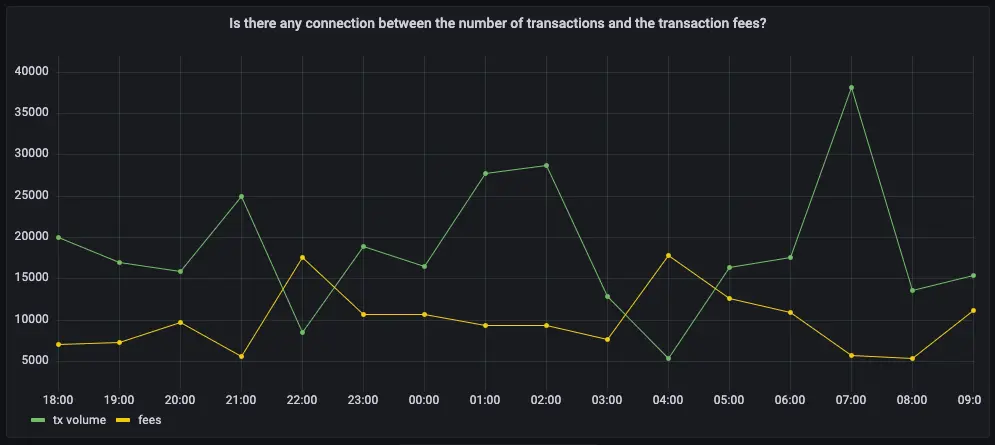
Is there any connection between the number of transactions and the transaction fees?

Transaction fees are a major concern for blockchain users. If a blockchain is too expensive, you might not want to use it. This query shows you whether there’s any correlation between the number of Bitcoin transactions and the fees. The time range for this analysis is the last 2 days.

If you choose to visualize the query in Grafana, you can see the average transaction volume and the average fee per transaction, over time. These trends might help you decide whether to submit a transaction now or wait a few days for fees to decrease.

1. Connect to the that contains the Bitcoin dataset.

2. At the psql prompt, use this query to average transaction volume and the fees from the one_hour_transactions :

   SELECT
    bucket AS "time",
    tx_count as "tx volume",
    average(stats_fee_sat) as fees
   FROM one_hour_transactions
   WHERE bucket > date_add('2023-11-22 00:00:00+00', INTERVAL '-2 days')
   ORDER BY 1;
   

3. The data you get back looks a bit like this:

           time          | tx volume |        fees
   ------------------------+-----------+--------------------
   2023-11-20 01:00:00+00 |      2602 | 105963.45810914681
   2023-11-20 02:00:00+00 |     33037 | 26686.814117504615
   2023-11-20 03:00:00+00 |     42077 | 22875.286546094067
   2023-11-20 04:00:00+00 |     46021 | 20280.843180287262
   2023-11-20 05:00:00+00 |     20828 | 24694.472969080085
   ...
   

4. To visualize this in Grafana:

   1. From the Dashboards page, click New and select New dashboard.
   2. Click Add visualization, then select the data source that connects to your .
   3. In the Queries section, change the Format to Time series and select Code.
   4. Type the query from the previous step and click Run query.

   

Does the transaction volume affect the BTC-USD rate?

In cryptocurrency trading, there’s a lot of speculation. You can adopt a data-based trading strategy by looking at correlations between blockchain metrics, such as transaction volume and the current exchange rate between Bitcoin and US Dollars.

If you choose to visualize the query in Grafana, you can see the average transaction volume, along with the BTC to US Dollar conversion rate.

1. Connect to the that contains the Bitcoin dataset.

2. At the psql prompt, use this query to return the trading volume and the BTC to US Dollar exchange rate:

   SELECT
    bucket AS "time",
    tx_count as "tx volume",
    total_fee_usd / (total_fee_sat*0.00000001) AS "btc-usd rate"
   FROM one_hour_transactions
   WHERE bucket > date_add('2023-11-22 00:00:00+00', INTERVAL '-2 days')
   ORDER BY 1;
   

3. The data you get back looks a bit like this:

             time          | tx volume |    btc-usd rate
   ------------------------+-----------+--------------------
    2023-06-13 08:00:00+00 |     20063 | 25975.888587931426
    2023-06-13 09:00:00+00 |     16984 |  25976.00446352126
    2023-06-13 10:00:00+00 |     15856 | 25975.988587014584
    2023-06-13 11:00:00+00 |     24967 |  25975.89166787936
    2023-06-13 12:00:00+00 |      8575 | 25976.004209699528
    ...
   

4. To visualize this in Grafana:

   1. From the Dashboards page, click New and select New dashboard.
   2. Click Add visualization, then select the data source that connects to your .
   3. In the Queries section, change the Format to Time series and select Code.
   4. Type the query from the previous step and click Run query.
   5. Under the panel options on the right, click Add field override > Fields with name, then choose btc-usd rate in the dropdown.
   6. Click Add override property, then select Axis > Placement and click Right.

   

Do more transactions in a block mean the block is more expensive to mine?

The number of transactions in a block can influence the overall block mining fee. For this analysis, a larger time frame is required, so increase the analyzed time range to 5 days.

If you choose to visualize the query in Grafana, you can see that the more transactions in a block, the higher the mining fee becomes.

1. Connect to the that contains the Bitcoin dataset.

2. At the psql prompt, use this query to return the number of transactions in a block, compared to the mining fee:

   SELECT
    bucket as "time",
    avg(tx_count) AS transactions,
    avg(block_fee_sat)*0.00000001 AS "mining fee"
   FROM one_hour_blocks
   WHERE bucket > date_add('2023-11-22 00:00:00+00', INTERVAL '-5 days')
   GROUP BY bucket
   ORDER BY 1;
   

3. The data you get back looks a bit like this:

             time          |     transactions      |       mining fee
   ------------------------+-----------------------+------------------------
    2023-06-10 08:00:00+00 | 2322.2500000000000000 | 0.29221418750000000000
    2023-06-10 09:00:00+00 | 3305.0000000000000000 | 0.50512649666666666667
    2023-06-10 10:00:00+00 | 3011.7500000000000000 | 0.44783255750000000000
    2023-06-10 11:00:00+00 | 2874.7500000000000000 | 0.39303009500000000000
    2023-06-10 12:00:00+00 | 2339.5714285714285714 | 0.25590717142857142857
   

4. To visualize this in Grafana:

   1. From the Dashboards page, click New and select New dashboard.
   2. Click Add visualization, then select the data source that connects to your .
   3. In the Queries section, change the Format to Time series and select Code.
   4. Type the query from the previous step and click Run query.
   5. Under the panel options on the right, click Add field override > Fields with name, then choose mining fee in the dropdown.
   6. Click Add override property, then select Axis > Placement and click Right.

   

You can extend this analysis to find if there is the same correlation between block weight and mining fee. More transactions should increase the block weight, and boost the miner fee as well.

If you choose to visualize the query in Grafana, you can see the same kind of high correlation between block weight and mining fee. The relationship weakens when the block weight gets close to its maximum value, which is 4 million weight units, in which case it’s impossible for a block to include more transactions.

1. Connect to the that contains the Bitcoin dataset.

2. At the psql prompt, use this query to return the block weight, compared to the mining fee:

   SELECT
    bucket as "time",
    avg(block_weight) as "block weight",
    avg(block_fee_sat*0.00000001) as "mining fee"
   FROM one_hour_blocks
   WHERE bucket > date_add('2023-11-22 00:00:00+00', INTERVAL '-5 days')
   group by bucket
   ORDER BY 1;
   

3. The data you get back looks a bit like this:

             time          |     block weight     |       mining fee
   ------------------------+----------------------+------------------------
    2023-06-10 08:00:00+00 | 3992809.250000000000 | 0.29221418750000000000
    2023-06-10 09:00:00+00 | 3991766.333333333333 | 0.50512649666666666667
    2023-06-10 10:00:00+00 | 3992918.250000000000 | 0.44783255750000000000
    2023-06-10 11:00:00+00 | 3991873.000000000000 | 0.39303009500000000000
    2023-06-10 12:00:00+00 | 3992934.000000000000 | 0.25590717142857142857
   ...
   

4. To visualize this in Grafana:

   1. From the Dashboards page, click New and select New dashboard.
   2. Click Add visualization, then select the data source that connects to your .
   3. In the Queries section, change the Format to Time series and select Code.
   4. Type the query from the previous step and click Run query.
   5. Under the panel options on the right, click Add field override > Fields with name, then choose mining fee in the dropdown.
   6. Click Add override property, then select Axis > Placement and click Right.

   

What percentage of the average miner’s revenue comes from fees compared to block rewards?

In the previous queries, you saw that mining fees are higher when block weights and transaction volumes are higher. This query analyzes the data from a different perspective. Miner revenue is not only made up of miner fees, it also includes block rewards for mining a new block. This reward is currently 6.25 BTC, and it gets halved every four years. This query looks at how much of a miner’s revenue comes from fees, compares to block rewards.

If you choose to visualize the query in Grafana, you can see that most miner revenue actually comes from block rewards. Fees never account for more than a few percentage points of overall revenue.

1. Connect to the that contains the Bitcoin dataset.

2. At the psql prompt, use this query to return coinbase transactions, along with the block fees and rewards:

   WITH coinbase AS (
      SELECT block_id, output_total AS coinbase_tx FROM transactions
      WHERE is_coinbase IS TRUE and time > date_add('2023-11-22 00:00:00+00', INTERVAL '-5 days')
   )
   SELECT
      bucket as "time",
      avg(block_fee_sat)*0.00000001 AS "fees",
      FIRST((c.coinbase_tx - block_fee_sat), bucket)*0.00000001 AS "reward"
   FROM one_hour_blocks b
   INNER JOIN coinbase c ON c.block_id = b.block_id
   GROUP BY bucket
   ORDER BY 1;
   

3. The data you get back looks a bit like this:

             time          |          fees          |   reward
   ------------------------+------------------------+------------
    2023-06-10 08:00:00+00 | 0.28247062857142857143 | 6.25000000
    2023-06-10 09:00:00+00 | 0.50512649666666666667 | 6.25000000
    2023-06-10 10:00:00+00 | 0.44783255750000000000 | 6.25000000
    2023-06-10 11:00:00+00 | 0.39303009500000000000 | 6.25000000
    2023-06-10 12:00:00+00 | 0.25590717142857142857 | 6.25000000
   ...
   

4. To visualize this in Grafana:

   1. From the Dashboards page, click New and select New dashboard.
   2. Click Add visualization, then select the data source that connects to your .
   3. In the Queries section, change the Format to Time series and select Code.
   4. Type the query from the previous step and click Run query.
   5. In the options panel, in the Graph styles section, for Stack series select 100%.

   

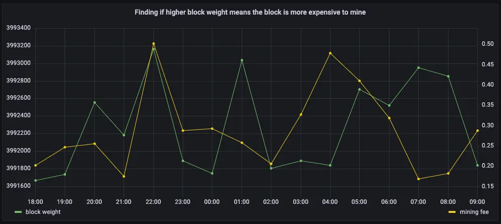
How does block weight affect miner fees?

You’ve already found that more transactions in a block mean it’s more expensive to mine. In this query, you ask if the same is true for block weights? The more transactions a block has, the larger its weight, so the block weight and mining fee should be tightly correlated. This query uses a 12-hour moving average to calculate the block weight and block mining fee over time.

If you choose to visualize the query in Grafana, you can see that the block weight and block mining fee are tightly connected. In practice, you can also see the four million weight units size limit. This means that there’s still room to grow for individual blocks, and they could include even more transactions.

1. Connect to the that contains the Bitcoin dataset.

2. At the psql prompt, use this query to return block weight, along with the block fees and rewards:

   WITH stats AS (
      SELECT
          bucket,
          stats_agg(block_weight, block_fee_sat) AS block_stats
      FROM one_hour_blocks
      WHERE bucket > date_add('2023-11-22 00:00:00+00', INTERVAL '-5 days')
      GROUP BY bucket
   )
   SELECT
      bucket as "time",
      average_y(rolling(block_stats) OVER (ORDER BY bucket RANGE '12 hours' PRECEDING)) AS "block weight",
      average_x(rolling(block_stats) OVER (ORDER BY bucket RANGE '12 hours' PRECEDING))*0.00000001 AS "mining fee"
   FROM stats
   ORDER BY 1;
   

3. The data you get back looks a bit like this:

             time          |    block weight    |     mining fee
   ------------------------+--------------------+---------------------
    2023-06-10 09:00:00+00 | 3991766.3333333335 |  0.5051264966666666
    2023-06-10 10:00:00+00 | 3992424.5714285714 | 0.47238710285714286
    2023-06-10 11:00:00+00 |            3992224 | 0.44353000909090906
    2023-06-10 12:00:00+00 |  3992500.111111111 | 0.37056557222222225
    2023-06-10 13:00:00+00 |         3992446.65 | 0.39728022799999996
   ...
   

4. To visualize this in Grafana:

   1. From the Dashboards page, click New and select New dashboard.
   2. Click Add visualization, then select the data source that connects to your .
   3. In the Queries section, change the Format to Time series and select Code.
   4. Type the query from the previous step and click Run query.
   5. Under the panel options on the right, click Add field override > Fields with name, then choose mining fee in the dropdown.
   6. Click Add override property, then select Axis > Placement and click Right.

   

What’s the average miner revenue per block?

In this final query, you analyze how much revenue miners actually generate by mining a new block on the blockchain, including fees and block rewards. To make the analysis more interesting, add the Bitcoin to US Dollar exchange rate, and increase the time range.

1. Connect to the that contains the Bitcoin dataset.

2. At the psql prompt, use this query to return the average miner revenue per block, with a 12-hour moving average:

   SELECT
      bucket as "time",
      average_y(rolling(stats_miner_revenue) OVER (ORDER BY bucket RANGE '12 hours' PRECEDING))*0.00000001 AS "revenue in BTC",
       average_x(rolling(stats_miner_revenue) OVER (ORDER BY bucket RANGE '12 hours' PRECEDING)) AS "revenue in USD"
   FROM one_hour_coinbase
   WHERE bucket > date_add('2023-11-22 00:00:00+00', INTERVAL '-5 days')
   ORDER BY 1;
   

3. The data you get back looks a bit like this:

             time          |   revenue in BTC   |   revenue in USD
   ------------------------+--------------------+--------------------
    2023-06-09 14:00:00+00 |       6.6732841925 |        176922.1133
    2023-06-09 15:00:00+00 |  6.785046736363636 |  179885.1576818182
    2023-06-09 16:00:00+00 |       6.7252952905 | 178301.02735000002
    2023-06-09 17:00:00+00 |  6.716377454814815 |  178064.5978074074
    2023-06-09 18:00:00+00 |    6.7784206471875 |   179709.487309375
   ...
   

4. To visualize this in Grafana:

   1. From the Dashboards page, click New and select New dashboard.
   2. Click Add visualization, then select the data source that connects to your .
   3. In the Queries section, change the Format to Time series and select Code.
   4. Type the query from the previous step and click Run query.
   5. Under the panel options on the right, click Add field override > Fields with name, then choose revenue in USD in the dropdown.
   6. Click Add override property, then select Axis > Placement and click Right.