Analyze financial tick data

Store financial tick data and create candlestick views for real-time analysis of price changes

The financial industry is extremely data-heavy and relies on real-time and historical data for decision-making, risk assessment, fraud detection, and market analysis. simplifies management of these large volumes of data, while also providing you with meaningful analytical insights and optimizing storage costs.

To analyze financial data, you can chart the open, high, low, close, and volume (OHLCV) information for a financial asset. Using this data, you can create candlestick charts that make it easier to analyze the price changes of financial assets over time. You can use candlestick charts to examine trends in stock, cryptocurrency, or NFT prices.

In this tutorial, you use real raw financial data provided by Twelve Data, create an aggregated candlestick view, query the aggregated data, and visualize the data in Grafana.

This tutorial covers:

1. Ingest data into a : load data from Twelve Data into your database.
2. Query your dataset: create candlestick views, query the aggregated data, and visualize the data in Grafana.

Prerequisites

To follow the steps on this page:

• Create a target with Real-time analytics enabled.

  You need your connection details. This procedure also works for .

• Install and run self-managed Grafana, or sign up for Grafana Cloud.

This tutorial uses a dataset that contains second-by-second trade data for the most-traded crypto-assets. You optimize this time-series data in a called crypto_ticks. You also create a separate table of asset symbols in a regular table named crypto_assets.

OHLCV data and candlestick charts

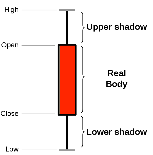
The financial sector regularly uses candlestick charts to visualize the price change of an asset. Each candlestick represents a time period, such as one minute or one hour, and shows how the asset’s price changed during that time.

Candlestick charts are generated from the open, high, low, close, and volume data for each financial asset during the time period. This is often abbreviated as OHLCV:

• Open: opening price
• High: highest price
• Low: lowest price
• Close: closing price
• Volume: volume of transactions

is well suited to storing and analyzing financial candlestick data, and many community members use it for exactly this purpose. Check out these stories from some community members:

• How Trading Strategy built a data stack for crypto quant trading
• How Messari uses data to open the cryptoeconomy to everyone
• How I power a (successful) crypto trading bot with

Optimize time-series data in a hypertable

s are tables in that automatically partition your time-series data by time. Time-series data represents the way a system, process, or behavior changes over time. s enable to work efficiently with time-series data. Each is made up of child tables called chunks. Each chunk is assigned a range of time, and only contains data from that range. When you run a query, identifies the correct chunk and runs the query on it, instead of going through the entire table.

is the hybrid row-columnar storage engine in used by s. Traditional databases force a trade-off between fast inserts (row-based storage) and efficient analytics (columnar storage). eliminates this trade-off, allowing real-time analytics without sacrificing transactional capabilities.

dynamically stores data in the most efficient format for its lifecycle:

• Row-based storage for recent data: the most recent chunk (and possibly more) is always stored in the , ensuring fast inserts, updates, and low-latency single record queries. Additionally, row-based storage is used as a writethrough for inserts and updates to columnar storage.
• Columnar storage for analytical performance: chunks are automatically compressed into the , optimizing storage efficiency and accelerating analytical queries.

Unlike traditional columnar databases, allows data to be inserted or modified at any stage, making it a flexible solution for both high-ingest transactional workloads and real-time analytics—within a single database.

Because is 100% , you can use all the standard tables, indexes, stored procedures, and other objects alongside your s. This makes creating and working with s similar to standard .

1. Connect to your

   In open an SQL editor. You can also connect to your service using psql.

2. Create a to store the real-time cryptocurrency data

   Create a for your time-series data using CREATE TABLE. For efficient queries on data in the , remember to segmentby the column you will use most often to filter your data:

   CREATE TABLE crypto_ticks (
       "time" TIMESTAMPTZ,
       symbol TEXT,
       price DOUBLE PRECISION,
       day_volume NUMERIC
   ) WITH (
      tsdb.hypertable,
      tsdb.segmentby='symbol',
      tsdb.orderby='time DESC'
   );
   

   When you create a using CREATE TABLE … WITH …, the default partitioning column is automatically the first column with a timestamp data type. Also, creates a columnstore policy that automatically converts your data to the , after an interval equal to the value of the chunk_interval, defined through compress_after in the policy. This columnar format enables fast scanning and aggregation, optimizing performance for analytical workloads while also saving significant storage space. In the conversion, s are compressed by up to 98%, and organized for efficient, large-scale queries.

   You can customize this policy later using alter_job. However, to change after or created_before, the compression settings, or the the policy is acting on, you must remove the columnstore policy and add a new one.

   You can also manually convert s in a to the .

Create a standard Postgres table for relational data

When you have relational data that enhances your time-series data, store that data in standard relational tables.

1. Add a table to store the asset symbol and name in a relational table

   CREATE TABLE crypto_assets (
       symbol TEXT UNIQUE,
       "name" TEXT
   );
   

You now have two tables within your . A hypertable named crypto_ticks, and a normal table named crypto_assets.

Load financial data

This tutorial uses real-time cryptocurrency data, also known as tick data, from Twelve Data. To ingest data into the tables that you created, you need to download the dataset, then upload the data to your .

1. Unzip crypto_sample.zip to a <local folder>.

   This test dataset contains second-by-second trade data for the most-traded crypto-assets and a regular table of asset symbols and company names.

   To import up to 100GB of data directly from your current -based database, migrate with downtime using native tooling. To seamlessly import 100GB-10TB+ of data, use the live migration tooling supplied by . To add data from non- data sources, see Import and ingest data.

2. In Terminal, navigate to <local folder> and connect to your .

   psql -d "postgres://<username>:<password>@<host>:<port>/<database-name>"
   

   The connection information for a is available in the file you downloaded when you created it.

3. At the psql prompt, use the COPY command to transfer data into your . If the .csv files aren’t in your current directory, specify the file paths in these commands:

   \COPY crypto_ticks FROM 'tutorial_sample_tick.csv' CSV HEADER;
   
   \COPY crypto_assets FROM 'tutorial_sample_assets.csv' CSV HEADER;
   

   Because there are millions of rows of data, the COPY process could take a few minutes depending on your internet connection and local client resources.

Query the data

Turning raw, real-time tick data into aggregated candlestick views is a common task for users who work with financial data. includes hyperfunctions that you can use to store and query your financial data more easily. Hyperfunctions are SQL functions within that make it easier to manipulate and analyze time-series data in with fewer lines of code.

There are three hyperfunctions that are essential for calculating candlestick values: time_bucket(), FIRST(), and LAST(). The time_bucket() hyperfunction helps you aggregate records into buckets of arbitrary time intervals based on the timestamp value. FIRST() and LAST() help you calculate the opening and closing prices. To calculate highest and lowest prices, you can use the standard aggregate functions MIN and MAX.

In , the most efficient way to create candlestick views is to use continuous aggregates. In this tutorial, you create a for a candlestick time bucket, and then query the aggregate with different refresh policies. Finally, you can use Grafana to visualize your data as a candlestick chart.

Create a continuous aggregate

To look at OHLCV values, the most effective way is to create a . In this tutorial, you create a to aggregate data for each day. You then set the aggregate to refresh every day, and to aggregate the last two days’ worth of data.

1. Connect to the that contains the Twelve Data cryptocurrency dataset.

2. At the psql prompt, create the to aggregate data every day:

   CREATE MATERIALIZED VIEW one_day_candle
   WITH (timescaledb.continuous) AS
       SELECT
           time_bucket('1 day', time) AS bucket,
           symbol,
           FIRST(price, time) AS "open",
           MAX(price) AS high,
           MIN(price) AS low,
           LAST(price, time) AS "close",
           LAST(day_volume, time) AS day_volume
       FROM crypto_ticks
       GROUP BY bucket, symbol;
   

   When you create the , it refreshes by default.

3. Set a refresh policy to update the every day, if there is new data available in the for the last two days:

   SELECT add_continuous_aggregate_policy('one_day_candle',
       start_offset => INTERVAL '3 days',
       end_offset => INTERVAL '1 day',
       schedule_interval => INTERVAL '1 day');
   

Query the continuous aggregate

When you have your set up, you can query it to get the OHLCV values.

1. Connect to the that contains the Twelve Data cryptocurrency dataset.

2. At the psql prompt, use this query to select all Bitcoin OHLCV data for the past 14 days, by time bucket:

   SELECT * FROM one_day_candle
   WHERE symbol = 'BTC/USD' AND bucket >= NOW() - INTERVAL '14 days'
   ORDER BY bucket;
   

   The result of the query looks like this:

            bucket         | symbol  |  open   |  high   |   low   |  close  | day_volume
   ------------------------+---------+---------+---------+---------+---------+------------
    2022-11-24 00:00:00+00 | BTC/USD |   16587 | 16781.2 | 16463.4 | 16597.4 |      21803
    2022-11-25 00:00:00+00 | BTC/USD | 16597.4 | 16610.1 | 16344.4 | 16503.1 |      20788
    2022-11-26 00:00:00+00 | BTC/USD | 16507.9 | 16685.5 | 16384.5 | 16450.6 |      12300
   

Connect Grafana to Tiger Cloud

To visualize the results of your queries, enable Grafana to read the data in your :

1. Log in to Grafana

   In your browser, log in to either:

   • Self-hosted Grafana: at http://localhost:3000/. The default credentials are admin, admin.
   • Grafana Cloud: use the URL and credentials you set when you created your account.

2. Add your as a data source

   1. Open Connections > Data sources, then click Add new data source.

   2. Select PostgreSQL from the list.

   3. Configure the connection:

      • Host URL, Database name, Username, and Password

        Configure using your connection details. Host URL is in the format <host>:<port>.

      • TLS/SSL Mode: select require.

      • PostgreSQL options: enable TimescaleDB.

      • Leave the default setting for all other fields.

   4. Click Save & test.

   Grafana checks that your details are set correctly.

Graph OHLCV data

When you have extracted the raw OHLCV data, you can use it to graph the result in a candlestick chart, using Grafana.

1. In Grafana, from the Dashboards page, click New and select New dashboard.

2. Click Add visualization, then select the data source that connects to your and the Candlestick visualization type in the top right.

3. In the Queries section, select Code and paste the query you used to get the OHLCV values:

   SELECT * FROM one_day_candle
   WHERE symbol = 'BTC/USD' AND bucket >= NOW() - INTERVAL '14 days'
   ORDER BY bucket;
   

4. Adjust elements of the table as required, and click Apply to save your graph to the dashboard.